Part I · Foundations Week 1 Published dp.py test_dp.py

Markov Decision Processes and Dynamic Programming

The finite MDP, the Bellman expectation and optimality equations, and the gamma-contraction that makes value iteration and policy iteration converge — dynamic programming as the spine the rest of the curriculum returns to.

Markov Decision Processes and Dynamic Programming

Where we are. This is the first chapter, and it states the object the whole curriculum orbits: the finite Markov decision process and the two equations that pin down optimal behaviour in it. The claim is small and load-bearing — the optimal value function is the unique fixed point of a $\discount$ -contraction, and value iteration and policy iteration are two ways of reaching that fixed point. Everything later — LQR, MPC, model-based and model-free RL — computes, approximates, or learns this same fixed point when the MDP is too large, too continuous, or unknown.

Chapter 1 — at a glance

Goal. Define the finite MDP; derive the Bellman expectation and optimality equations; prove the Bellman operators are $\discount$ -contractions; read value iteration and policy iteration off the contraction.

Reading time. ~45 minutes; ~75 with the proofs and exercises.

Key insight — the DP bridge. A value function is a fixed point. The optimality operator $\bellmanopt$ contracts the sup-norm by $\discount$ , so by the Banach fixed-point theorem it has exactly one fixed point, $\optvaluefn$ , and every iterate converges to it geometrically. This one fact is the spine of the book: LQR (Ch. 13) is this fixed point in closed form on linear-quadratic dynamics; MPC (Ch. 15) is this fixed point recomputed online over a finite horizon; model-free RL (Ch. 5+) is stochastic approximation of the same operator from samples.

Notation and conventions

We use the case convention of Sutton & Barto Sutton & Barto (2018) throughout: lowercase names a true object we want ( $\valuefn_\policy$ ), and uppercase names an estimate we hold and update ( $V_k$ ).

| Symbol | Meaning | |---|---| | $\statespace,\ \actionspace$ | finite state and action sets; $\lvert\statespace\rvert, \lvert\actionspace\rvert < \infty$ | | $\transition(s',r \mid s,a)$ | dynamics — joint probability of next state $s'$ and reward $r$ | | $\policy(a \mid s)$ | policy — probability of action $a$ in state $s$ | | $\discount \in [0,1)$ | discount factor (strict inequality is load-bearing) | | $\valuefn_\policy,\ \qfn_\policy$ | state- and action-value functions of $\policy$ (true) | | $\optvaluefn,\ \optqfn$ | optimal value functions | | $V_k \in \R^{\statespace}$ | the $k$ -th value iterate (an estimate of $\optvaluefn$ ) | | $\bellman^\policy,\ \bellmanopt$ | Bellman expectation / optimality operators | | $\norm{\cdot}_\infty$ | sup norm on $\R^{\statespace}$ : $\norm{v}_\infty \defeq \max_{s} \lvert v(s)\rvert$ |

A value function on a finite state set is a vector in $\R^{\statespace}$ , a point in $\lvert\statespace\rvert$ -dimensional space.

The operators below move that point around, and “solving the MDP” means finding the one point they hold still.

The finite Markov decision process

A Markov decision process is a controlled Markov chain: at each step the agent sees a state, picks an action, and the environment returns a reward and a next state, with the Markov property that the future depends on the past only through the current state.

Definition 1.1 (Finite MDP).

A finite Markov decision process is a tuple $(\statespace, \actionspace, \transition, \discount)$ with $\statespace, \actionspace$ finite, discount $\discount \in [0,1)$ , and dynamics

\transition(s',r \mid s,a) \defeq \Prob\!\big(S_{t+1}=s',\, R_{t+1}=r \,\big|\, S_t=s,\, A_t=a\big),

a probability distribution over $(s',r)$ for each $(s,a)$ . We write the state-transition kernel and expected reward as the marginals

\transition(s' \mid s,a) \defeq \sum_{r} \transition(s',r \mid s,a), \qquad \reward(s,a) \defeq \sum_{s',r} \transition(s',r \mid s,a)\, r .

The Markov property is the modelling commitment that earns us everything that follows: because the next state and reward depend only on $(S_t, A_t)$ , a value function needs only one argument — the current state — and the recursion below closes on itself.

The canonical reference for the finite-MDP formalism and its solution methods is Puterman Puterman (1994) ; the founding treatment of the underlying optimization principle is Bellman Bellman (1957) .

Definition 1.2 (Policy and discounted return).

A (stationary) policy $\policy(a\mid s)$ is a distribution over actions for each state. Acting under $\policy$ produces a trajectory $S_0, A_0, R_1, S_1, A_1, R_2, \dots$ , and the discounted return from time $t$ is

G_t \defeq \sum_{k=0}^{\infty} \discount^{k} R_{t+k+1}.

Because rewards are bounded on a finite MDP and $\discount<1$ , the series converges absolutely, with $\lvert G_t\rvert \le R_{\max}/(1-\discount)$ where $R_{\max} \defeq \max_{s,a}\lvert\reward(s,a)\rvert$ .

Value functions

A value function answers one question: starting here and acting under $\policy$ , how much discounted reward do I expect? The state-value fixes the starting state; the action-value also fixes the first action.

Definition 1.3 (State- and action-value functions).

For a policy $\policy$ , the state-value and action-value functions are

\valuefn_\policy(s) \defeq \E_\policy\!\big[\,G_t \,\big|\, S_t = s\,\big], \qquad \qfn_\policy(s,a) \defeq \E_\policy\!\big[\,G_t \,\big|\, S_t = s,\, A_t = a\,\big],

where $\E_\policy$ averages over trajectories generated by $\policy$ and $\transition$ . The two are linked by $\valuefn_\policy(s) = \sum_a \policy(a\mid s)\,\qfn_\policy(s,a)$ .

The Bellman expectation equation

Everything recursive about value functions comes from one move: split the return into the immediate reward and the discounted return from the next state, then condition on what happens in one step. That conditioning is the law of total expectation, the single most-used tool in RL theory.

Theorem 1.1 (Bellman expectation equation).

For every policy $\policy$ and state $s$ ,

\valuefn_\policy(s) = \sum_{a} \policy(a\mid s) \sum_{s',r} \transition(s',r\mid s,a) \big[\, r + \discount\, \valuefn_\policy(s') \,\big].

Proof.

Start from the definition and peel off one step of the return, $G_t = R_{t+1} + \discount\, G_{t+1}$ :

\begin{aligned} \valuefn_\policy(s) &= \E_\policy[\,R_{t+1} + \discount\, G_{t+1} \mid S_t = s\,] && \text{(Def. 1.3; unroll }G_t\text{)} \\ &= \sum_{a} \policy(a\mid s) \sum_{s',r} \transition(s',r\mid s,a)\, \E_\policy[\,r + \discount\, G_{t+1} \mid S_{t+1}=s'\,] && \text{(law of total expectation, condition on }A_t, S_{t+1}, R_{t+1}\text{)} \\ &= \sum_{a} \policy(a\mid s) \sum_{s',r} \transition(s',r\mid s,a)\, \big[\, r + \discount\, \E_\policy[\,G_{t+1}\mid S_{t+1}=s'\,] \,\big] && \text{(linearity; }r\text{ is fixed once we condition)} \\ &= \sum_{a} \policy(a\mid s) \sum_{s',r} \transition(s',r\mid s,a)\, \big[\, r + \discount\, \valuefn_\policy(s') \,\big] && \text{(Markov property: }\E_\policy[G_{t+1}\mid S_{t+1}=s']=\valuefn_\policy(s')\text{).} \end{aligned}

The Markov property is what licenses the last line: the expected return from $t+1$ onward depends on the past only through $S_{t+1}=s'$ . $\qquad\blacksquare$

Read as a system of $\lvert\statespace\rvert$ linear equations in the unknowns $\{\valuefn_\policy(s)\}$ , the Bellman expectation equation defines $\valuefn_\policy$ . Collecting it into a single map on $\R^{\statespace}$ gives the operator we will iterate.

Definition 1.4 (Bellman expectation operator).

The Bellman expectation operator $\bellman^\policy : \R^{\statespace} \to \R^{\statespace}$ acts on a value vector $v$ by

(\bellman^\policy v)(s) \defeq \sum_{a} \policy(a\mid s) \sum_{s',r} \transition(s',r\mid s,a)\,\big[\, r + \discount\, v(s') \,\big] = \reward_\policy(s) + \discount \sum_{s'} \transition_\policy(s'\mid s)\, v(s'),

where $\reward_\policy(s) \defeq \sum_a \policy(a\mid s)\reward(s,a)$ and $\transition_\policy(s'\mid s) \defeq \sum_a \policy(a\mid s)\transition(s'\mid s,a)$ . By Theorem 1.1, $\valuefn_\policy$ is a fixed point: $\bellman^\policy \valuefn_\policy = \valuefn_\policy$ .

In vector form $\bellman^\policy v = \reward_\policy + \discount P_\policy v$ with $P_\policy$ the $\lvert\statespace\rvert\times\lvert\statespace\rvert$ transition matrix — an affine map, so its fixed point solves the linear system $(I - \discount P_\policy)\valuefn_\policy = \reward_\policy$ . We will use that closed form for policy evaluation below.

Optimality: the Bellman optimality equation

So far $\policy$ was fixed. Optimal control asks for the best achievable value, and — remarkably — a single policy attains it simultaneously in every state.

Definition 1.5 (Optimal value functions and optimal policy).

The optimal value functions are

\optvaluefn(s) \defeq \max_{\policy} \valuefn_\policy(s), \qquad \optqfn(s,a) \defeq \max_{\policy} \qfn_\policy(s,a),

the maxima taken pointwise over all policies. A policy $\policy_*$ is optimal if $\valuefn_{\policy_*} = \optvaluefn$ .

Theorem 1.2 (Bellman optimality equation).

The optimal state-value function satisfies, for every $s$ ,

\optvaluefn(s) = \max_{a \in \actionspace} \Big[\, \reward(s,a) + \discount \sum_{s'} \transition(s'\mid s,a)\, \optvaluefn(s') \,\Big] = \max_{a} \optqfn(s,a),

and a policy is optimal iff it is greedy with respect to $\optvaluefn$ — i.e. in each state it puts all mass on actions attaining the maximum.

Proof.

We argue from Bellman’s principle of optimality Bellman (1957) , assuming for now that $\optvaluefn$ is well defined; the next section discharges that assumption — Theorem 1.3 and Corollary 1.1 establish existence and uniqueness without using this equation, so the reasoning is not circular. An optimal trajectory’s tail is itself optimal from the state it reaches. Fix $s$ . Any policy chooses a first action (or distribution over them) and then continues; its value cannot exceed taking the best first action $a$ and continuing optimally, which is exactly $\max_a [\reward(s,a) + \discount \sum_{s'} \transition(s'\mid s,a)\,\optvaluefn(s')]$ — so $\optvaluefn(s)$ is at most the right-hand side. Conversely, the policy that takes the maximizing $a$ and then follows an optimal policy achieves that value, so $\optvaluefn(s)$ is at least the right-hand side. Equality gives the optimality equation; the two bounds coincide exactly when the policy is greedy for $\optvaluefn$ . $\qquad\blacksquare$

The $\max$ over actions makes this equation nonlinear — there is no matrix inverse to solve it.

That nonlinearity is the entire reason we iterate rather than solve. Bertsekas Bertsekas (2017) develops the resulting theory abstractly as fixed-point iteration of monotone contraction operators; we specialize it to finite MDPs.

Definition 1.6 (Bellman optimality operator).

The Bellman optimality operator $\bellmanopt : \R^{\statespace} \to \R^{\statespace}$ is

(\bellmanopt v)(s) \defeq \max_{a \in \actionspace} \Big[\, \reward(s,a) + \discount \sum_{s'} \transition(s'\mid s,a)\, v(s') \,\Big].

Theorem 1.2 says $\optvaluefn$ is a fixed point: $\bellmanopt \optvaluefn = \optvaluefn$ .

The contraction that makes it all work

Both operators share one property, and it is the technical heart of the chapter. Recall a map $T$ is a $\discount$ -contraction in a norm if $\norm{Tu - Tv} \le \discount\,\norm{u-v}$ for all $u,v$ .

Theorem 1.3 (Bellman operators are sup-norm contractions).

For any $u, v \in \R^{\statespace}$ ,

\norm{\bellmanopt u - \bellmanopt v}_\infty \le \discount\,\norm{u - v}_\infty, \qquad \norm{\bellman^\policy u - \bellman^\policy v}_\infty \le \discount\,\norm{u - v}_\infty .

Both operators are $\discount$ -contractions on $(\R^{\statespace}, \norm{\cdot}_\infty)$ .

Proof.

We prove it for $\bellmanopt$ ; the $\bellman^\policy$ case is Exercise 1 (it is easier — no $\max$ ). The bound takes four short steps, each labelled with the rule it uses. Fix a state $s$ and write $Q_w(s,a) \defeq \reward(s,a) + \discount \sum_{s'} \transition(s'\mid s,a)\,w(s')$ , so $(\bellmanopt w)(s) = \max_a Q_w(s,a)$ . The one inequality we need is that the $\max$ is nonexpansive: $\lvert \max_a f(a) - \max_a g(a)\rvert \le \max_a \lvert f(a)-g(a)\rvert$ . Then

\begin{aligned} \big\lvert (\bellmanopt u)(s) - (\bellmanopt v)(s) \big\rvert &= \big\lvert \max_a Q_u(s,a) - \max_a Q_v(s,a) \big\rvert && \text{(definition)} \\ &\le \max_a \big\lvert Q_u(s,a) - Q_v(s,a) \big\rvert && \text{($\max$ is nonexpansive)} \\ &= \max_a\ \discount \Big\lvert \textstyle\sum_{s'} \transition(s'\mid s,a)\,\big(u(s') - v(s')\big) \Big\rvert && \text{($\reward(s,a)$ cancels)} \\ &\le \discount \max_a \sum_{s'} \transition(s'\mid s,a)\, \big\lvert u(s') - v(s') \big\rvert && \text{(triangle inequality)} \\ &\le \discount \max_a \sum_{s'} \transition(s'\mid s,a)\, \norm{u - v}_\infty = \discount\, \norm{u - v}_\infty && \text{($\textstyle\sum_{s'} \transition(s'\mid s,a) = 1$).} \end{aligned}

The bound is uniform in $s$ , so taking the max over $s$ on the left gives $\norm{\bellmanopt u - \bellmanopt v}_\infty \le \discount\norm{u-v}_\infty$ . $\qquad\blacksquare$

The discount $\discount < 1$ is doing all the work: it is literally the contraction modulus. With $\discount = 1$ the bound is vacuous and the fixed-point theory needs extra structure (proper policies, average cost) — the subject of later asides.

Corollary 1.1 (Unique value functions and geometric convergence).

Because $(\R^{\statespace}, \norm{\cdot}_\infty)$ is complete and both operators are $\discount$ -contractions, the Banach fixed-point theorem gives:

$\bellman^\policy$ has a unique fixed point, necessarily $\valuefn_\policy$ ; and $\bellmanopt$ has a unique fixed point, necessarily $\optvaluefn$ . In particular $\optvaluefn$ exists and is unique, and an optimal stationary policy exists (any greedy policy for $\optvaluefn$ — the policy-improvement theorem below confirms such a policy attains $\optvaluefn$ ).
The iterates $V_{k+1} \defeq \bellmanopt V_k$ converge to $\optvaluefn$ from any start $V_0$ , geometrically: $\norm{V_k - \optvaluefn}_\infty \le \discount^{k}\, \norm{V_0 - \optvaluefn}_\infty .$

This corollary is the payoff. It converts an existence question (“is there a best policy?”) into a convergent algorithm (“iterate the operator”), and it tells us the error shrinks by a factor $\discount$ every sweep.

Value iteration

Value iteration is now nothing more than iterate $\bellmanopt$ to its fixed point.

V ← 0  (any initial vector in ℝ^𝒮)
repeat:
    V ← 𝒯* V            # one sweep of the optimality operator
until ‖ΔV‖∞ < ε(1−γ)/γ   # stopping rule, justified below
return V, and the greedy policy π(s) = argmax_a [ r(s,a) + γ Σ p(s'|s,a) V(s') ]

Corollary 1.1 guarantees convergence. The stopping rule deserves a word: a small Bellman residual $\norm{V_{k+1} - V_k}_\infty$ bounds the true error, because

\norm{V_{k} - \optvaluefn}_\infty \le \frac{\discount}{1-\discount}\,\norm{V_{k} - V_{k-1}}_\infty .

This telescopes from the contraction — write $V_k - \optvaluefn = \sum_{j\ge k}(V_{j+1} - V_j)$ and bound each term geometrically (Exercise 5). So stopping when $\norm{\Delta V}_\infty < \varepsilon(1-\discount)/\discount$ certifies $\norm{V - \optvaluefn}_\infty < \varepsilon$ — a guarantee we can check at runtime without knowing $\optvaluefn$ . The companion experiments/python/week01/dp.py implements exactly this loop with the explicit operator as a standalone function, as the roadmap’s Week-1 task asks.

Policy iteration

Value iteration improves the value every sweep and reads off a policy at the end. Policy iteration instead alternates two exact steps on the policy, and was Howard’s original 1960 algorithm Howard (1960) :

Policy evaluation. Given $\policy$ , solve the linear system $(I - \discount P_\policy)\,\valuefn_\policy = \reward_\policy$ for $\valuefn_\policy$ (the affine fixed point of $\bellman^\policy$ — Def. 1.4).
Policy improvement. Set $\policy'(s) = \argmax_a \qfn_\policy(s,a)$ , greedy w.r.t. the freshly evaluated values.

Repeat until the policy stops changing. The step that makes this work is:

Theorem 1.4 (Policy improvement theorem).

Let $\policy'$ be greedy with respect to $\valuefn_\policy$ , so that $\qfn_\policy(s, \policy'(s)) \ge \valuefn_\policy(s)$ for all $s$ . Then $\valuefn_{\policy'}(s) \ge \valuefn_\policy(s)$ for all $s$ , with strict improvement in some state unless $\policy$ is already optimal.

Proof.

Expand the greedy inequality and re-apply it along the trajectory:

\begin{aligned} \valuefn_\policy(s) &\le \qfn_\policy(s, \policy'(s)) && \text{(greedy choice)} \\ &= \E_{\policy'}\!\big[\, R_{t+1} + \discount\, \valuefn_\policy(S_{t+1}) \mid S_t = s \,\big] && \text{(definition of }\qfn_\policy\text{ under the first action }\policy'\text{)} \\ &\le \E_{\policy'}\!\big[\, R_{t+1} + \discount\, \qfn_\policy(S_{t+1}, \policy'(S_{t+1})) \mid S_t = s \,\big] && \text{(apply the greedy inequality at }S_{t+1}\text{)} \\ &\le \cdots \le \E_{\policy'}\!\Big[\, \textstyle\sum_{k\ge 0} \discount^{k} R_{t+k+1} \mid S_t = s \,\Big] = \valuefn_{\policy'}(s) && \text{(unroll; the tail telescopes to }\valuefn_{\policy'}\text{).} \end{aligned}

If no state improves strictly, the greedy inequality holds with equality everywhere, which is the Bellman optimality equation — so $\policy$ is already optimal. $\qquad\blacksquare$

Because the MDP is finite there are finitely many deterministic policies, each iteration strictly improves until none does, so policy iteration terminates at an exact optimum in finitely many steps. Value iteration and policy iteration are the two poles of what Sutton & Barto Sutton & Barto (2018) call generalized policy iteration: any interleaving of “make the value consistent with the policy” and “make the policy greedy for the value” converges to the same fixed point. Week 2 studies what happens between the poles — asynchronous, Gauss–Seidel, and prioritized sweeps.

The dynamic-programming bridge

The roadmap’s Week-1 writing prompt is to place the Bellman equation beside its continuous cousin. They are the same principle of optimality at different limits. Discretize time and state and the cost-to-go obeys the discrete Bellman recursion above; take the limit of vanishing time-step on a continuous state and the same recursion becomes the Hamilton–Jacobi–Bellman equation. Control flips the convention from maximizing reward to minimizing a running cost

\ell = -\reward

, with cost-to-go

J

; the stationary discounted HJB equation is

\rho\, J(x) = \min_{a}\Big[\, \ell(x,a) + \nabla J(x)^{\!\top} f(x,a) \,\Big], \qquad \rho = -\ln\discount,

whose $\rho J$ term is the continuous-time echo of the discount $\discount$ that drove the contraction above (set $\rho = 0$ for the undiscounted limit). Value iteration is the fixed-point solver for the discrete equation; the LQR Riccati recursion (Ch. 13) is the closed-form solver for the HJB equation when $f$ is linear and $\ell$ is quadratic. Holding this identity in view is the point of the whole curriculum: control theory and RL are two dialects for the same fixed point.

What’s next

Week 2 opens up the iteration itself: asynchronous and Gauss–Seidel value iteration, prioritized sweeping, real-time DP, and residual scheduling — the practical face of “iterate the contraction.”
Week 3 replaces the known model $\transition$ with sampled returns (Monte Carlo), the first step away from dynamic programming toward learning.

Exercises

(Prove) Show that the Bellman expectation operator $\bellman^\policy$ is a $\discount$ -contraction in $\norm{\cdot}_\infty$ . (This is the no- $\max$ case of Theorem 1.3.)

Solution
For any $s$ , $(\bellman^\policy u)(s) - (\bellman^\policy v)(s) = \discount \sum_{s'} \transition_\policy(s'\mid s)\,(u(s') - v(s'))$ since $\reward_\policy(s)$ cancels. Taking absolute values and using the triangle inequality with $\sum_{s'}\transition_\policy(s'\mid s)=1$ , $\lvert(\bellman^\policy u)(s) - (\bellman^\policy v)(s)\rvert \le \discount \sum_{s'}\transition_\policy(s'\mid s)\norm{u-v}_\infty = \discount\norm{u-v}_\infty$ . Maximizing over $s$ gives the claim. (No $\max$ -nonexpansiveness step is needed, because $\bellman^\policy$ is affine.)
(Derive) State and prove the Bellman expectation equation for the action-value $\qfn_\policy(s,a)$ .

Solution
Conditioning on the first transition and then the next action,
$\qfn_\policy(s,a) = \sum_{s',r}\transition(s',r\mid s,a)\Big[\,r + \discount \sum_{a'}\policy(a'\mid s')\,\qfn_\policy(s',a')\,\Big].$
The derivation is identical to Theorem 1.1 with the first action held fixed at $a$ and the recursion closing on $\qfn_\policy$ via $\valuefn_\policy(s') = \sum_{a'}\policy(a'\mid s')\qfn_\policy(s',a')$ .
(Compute) Take the two-state MDP $\statespace=\{A,B\}$ , actions $\{\text{stay},\text{switch}\}$ , $\discount=0.9$ , with deterministic dynamics: in $A$ , stay $\to A$ ( $r=0$ ) and switch $\to B$ ( $r=0$ ); in $B$ , stay $\to B$ ( $r=1$ ) and switch $\to A$ ( $r=0$ ). Evaluate the always-stay policy by solving $(I-\discount P_\policy)\valuefn_\policy = \reward_\policy$ .

Solution
Under always-stay, $P_\policy = I$ and $\reward_\policy = (0, 1)$ , so $(I - 0.9 I)\valuefn_\policy = (0,1)$ gives $0.1\,\valuefn_\policy = (0,1)$ , i.e. $\valuefn_\policy = (0, 10)$ . State $B$ self-loops collecting $1$ forever ( $1/(1-\discount)=10$ ); state $A$ self-loops collecting $0$ . This is the exact case the companion test asserts.
(Prove) Derive the geometric error bound of Corollary 1.1(2), $\norm{V_k - \optvaluefn}_\infty \le \discount^{k}\norm{V_0 - \optvaluefn}_\infty$ , from the contraction property and $\bellmanopt\optvaluefn=\optvaluefn$ .

Solution
$\norm{V_k - \optvaluefn}_\infty = \norm{\bellmanopt V_{k-1} - \bellmanopt \optvaluefn}_\infty \le \discount\norm{V_{k-1}-\optvaluefn}_\infty$ by Theorem 1.3 and the fixed-point identity. Iterating the inequality $k$ times gives the bound.
(Implement) Add the certified stopping rule to value iteration: stop when $\norm{\Delta V}_\infty < \varepsilon(1-\discount)/\discount$ and verify empirically that the returned $V$ satisfies $\norm{V-\optvaluefn}_\infty < \varepsilon$ on the two-state MDP (using the analytic $\optvaluefn=(9,10)$ ). Run against experiments/python/week01/dp.py.

Solution
The bound follows by writing $V_k - \optvaluefn = \sum_{j\ge k}(V_{j+1}-V_j)$ and bounding each term by the contraction: $\norm{V_{j+1}-V_j}_\infty \le \discount^{\,j-k}\norm{V_{k}-V_{k-1}}_\infty$ , a geometric series summing to $\frac{\discount}{1-\discount}\norm{\Delta V}_\infty$ . The companion’s value_iteration(..., tol=ε) implements this and its test asserts the resulting error is below $\varepsilon$ .
(Extend) Show the optimal value function is the solution of the linear program $\min_{v}\sum_s v(s)$ subject to $v(s) \ge \reward(s,a) + \discount \sum_{s'}\transition(s'\mid s,a)v(s')$ for all $s,a$ .

Solution
Feasibility means $v \ge \bellmanopt v$ pointwise; by monotonicity of $\bellmanopt$ this implies $v \ge \optvaluefn$ , so $\optvaluefn$ is the smallest feasible point and minimizing $\sum_s v(s)$ selects it. The constraints linearize the $\max$ (one inequality per action), turning the nonlinear optimality equation into an LP — the basis of the dual/occupancy-measure view revisited with safe RL in Week 25.

Companion code

The Week-1 companion lives at experiments/python/week01/ (the repo’s three-language convention). It is pure NumPy at the core — the algorithms and the correctness test carry no environment dependency — with an optional Gymnasium adapter for the canonical FrozenLake showcase.

dp.py — the Bellman optimality operator as an explicit function, plus value_iteration, policy_evaluation (exact linear solve), policy_improvement, and policy_iteration, all on a generic finite MDP (P, R, gamma).
test_dp.py — mathematical-correctness tests: convergence to the analytic $\optvaluefn=(9,10)$ on the two-state MDP of Exercise 3, the contraction inequality of Theorem 1.3, the fixed-point identity, the geometric bound, and VI/PI agreement (FrozenLake checks run only when gymnasium is installed).
frozenlake.py — builds (P, R, gamma) from gymnasium’s FrozenLake-v1 and runs VI and PI as a worked showcase.

# core algorithms + correctness tests (no Gymnasium needed)
PYTHONPATH=. pytest experiments/python/week01/test_dp.py -q

# canonical FrozenLake showcase (optional extra: pip install "gymnasium")
PYTHONPATH=. python experiments/python/week01/frozenlake.py

Part I · Foundations Week 2 Published async_dp.py test_async_dp.py

Asynchronous and Prioritized Dynamic Programming

Keeping the gamma-contraction but varying the schedule: asynchronous and Gauss–Seidel value iteration, prioritized sweeping, and real-time DP. Why the order of backups is free — monotonicity plus a constant-shift identity — and how update order and residual size set the practical convergence rate.

Asynchronous and Prioritized Dynamic Programming

Where we are. Chapter 1 proved that value iteration and policy iteration both reach the optimal value function because the Bellman operators are $\discount$ -contractions. Both methods share one extravagance: every sweep backs up every state, in lockstep, whether or not that state’s value has stopped moving. This chapter keeps the contraction and varies only the schedule — which states we back up, in what order, and using whose values. The load-bearing claim is that the order is nearly free: as long as every state is updated infinitely often, asynchronous dynamic programming converges to the same fixed point $\optvaluefn$ , and ordering the updates well — Gauss–Seidel, prioritized sweeping, real-time DP — buys large savings without touching the convergence theory.

Chapter 2 — at a glance

Goal. Define asynchronous and Gauss–Seidel value iteration; prove they converge using two structural properties (monotonicity and a constant-shift identity); read prioritized sweeping and real-time DP off the same theory; and quantify how update order and the discount set the number of backups.

Reading time. ~35 minutes; ~55 with the proof and exercises.

Key insight — the DP bridge. Synchronous value iteration is the Jacobi iteration for a nonlinear fixed-point system; Gauss–Seidel value iteration is its in-place cousin and prioritized sweeping its residual-ordered cousin — exactly the hierarchy classical numerical linear algebra builds for linear systems. The discount $\discount$ is again the load-bearing constant: it is the contraction modulus, and $1/(1-\discount)$ is the effective horizon that sets the iteration count.

Generalized policy iteration: the space between the poles

Chapter 1 closed by naming value iteration and policy iteration the two poles of generalized policy iteration (GPI): VI applies one optimality backup everywhere and reads off a greedy policy at the end; PI evaluates a policy exactly (a linear solve) and then improves it greedily. The methods in between truncate the evaluation. Modified policy iteration Puterman (1994) runs $m$ sweeps of the expectation operator $\bellman^\policy$ in place of the exact solve: $m=1$ recovers value iteration, $m\to\infty$ recovers policy iteration, and intermediate $m$ trades evaluation cost against the number of outer improvements. Sutton & Barto Sutton & Barto (2018) frame the entire family as two interacting processes — make the value consistent with the policy, make the policy greedy for the value — that converge to the same fixed point regardless of how finely they are interleaved.

This chapter relaxes a different lockstep: not how much we evaluate between improvements, but which states we touch on each pass and in what order.

Asynchronous value iteration

Synchronous value iteration computes the whole vector $\bellmanopt V_k$ from $V_k$ and only then overwrites — every state is backed up from the same old values. Asynchronous value iteration drops that barrier.

Definition 2.1 (Asynchronous value iteration).

Asynchronous value iteration maintains a single value vector $V$ and repeats: select a state $s$ and overwrite

V(s) \;\leftarrow\; (\bellmanopt V)(s) = \max_{a}\Big[\reward(s,a) + \discount \sum_{s'}\transition(s'\mid s,a)\,V(s')\Big],

using the current entries of $V$ — including any updated earlier in the pass. States may be visited in any order, subject only to the fairness condition that every state is selected infinitely often. The special case that sweeps the states in a fixed order $1,2,\dots,\lvert\statespace\rvert$ , each backup seeing the freshly written values of its predecessors, is Gauss–Seidel value iteration.

The synchronous operator of Chapter 1 reuses no in-pass information; Gauss–Seidel reuses all of it; general asynchronous iteration lives anywhere between. The question is whether dropping the barrier costs us the convergence guarantee. It does not, and the reason is two structural facts that cost one line each.

Why the order is free: monotonicity and the constant-shift identity

Proposition 2.1 (Monotonicity and constant-shift).

Let $T$ be either Bellman operator ( $\bellman^\policy$ or $\bellmanopt$ ). For all $u,v\in\R^{\statespace}$ and every constant $c\in\R$ , writing $\mathbf 1$ for the all-ones vector:

Monotonicity. If $u \le v$ componentwise, then $Tu \le Tv$ .
Constant-shift. $T(v + c\,\mathbf 1) = Tv + \discount c\,\mathbf 1$ .

Proof.

Both read off the backup $Q_v(s,a) \defeq \reward(s,a) + \discount\sum_{s'} \transition(s'\mid s,a)\,v(s')$ , of which $(\bellmanopt v)(s)=\max_a Q_v(s,a)$ and $(\bellman^\policy v)(s)=\sum_a\policy(a\mid s)Q_v(s,a)$ .

Monotonicity. If $u\le v$ then $\sum_{s'}\transition(s'\mid s,a)u(s') \le \sum_{s'}\transition(s'\mid s,a)v(s')$ because the transition weights are nonnegative; hence $Q_u(s,a)\le Q_v(s,a)$ for every $(s,a)$ , and taking the $\max$ (or the $\policy$ -average) over $a$ preserves the inequality.

Constant-shift. Since $\sum_{s'}\transition(s'\mid s,a)=1$ , replacing $v$ by $v+c\,\mathbf 1$ adds exactly $\discount c$ to every $Q_v(s,a)$ ; and $\max_a(x_a+\discount c)=\max_a x_a+\discount c$ (likewise for the average). $\qquad\blacksquare$

These two facts — and not the full contraction algebra — are what make asynchronous order irrelevant.

Theorem 2.1 (Asynchronous convergence).

Run asynchronous value iteration (Def. 2.1) from any $V_0$ , updating every state infinitely often. Then $V_k \to \optvaluefn$ . Moreover, grouping the schedule into rounds — a round ends once every state has been backed up at least once since the round began — the sup-norm error contracts by a factor $\discount$ per round:

\norm{V_{\text{after round } m} - \optvaluefn}_\infty \le \discount^{m}\, \norm{V_0 - \optvaluefn}_\infty .

Proof.

Let $c \defeq \norm{V_0-\optvaluefn}_\infty$ , so the iterate starts inside the box $\optvaluefn - c\,\mathbf 1 \le V_0 \le \optvaluefn + c\,\mathbf 1$ . Suppose at some moment $V$ lies in this box. Back up any state $s$ . By monotonicity and then constant-shift (Prop. 2.1), using $\bellmanopt\optvaluefn=\optvaluefn$ ,

(\bellmanopt V)(s) \le \big(\bellmanopt(\optvaluefn + c\,\mathbf 1)\big)(s) = \optvaluefn(s) + \discount c, \qquad (\bellmanopt V)(s) \ge \optvaluefn(s) - \discount c .

So the updated entry lands in the smaller box $[\optvaluefn(s)-\discount c,\, \optvaluefn(s)+\discount c]\subseteq[\optvaluefn(s)-c,\,\optvaluefn(s)+c]$ (as $\discount<1$ ). Two consequences: the iterate never leaves the original $c$ -box, and every state, once backed up, sits in the $\discount c$ -box. Crucially, later backups in the round still read values inside the original $c$ -box, so they too map into the $\discount c$ -box. Hence after one full round $\norm{V-\optvaluefn}_\infty\le\discount c$ . Applying the argument round by round gives $\discount^{m}c$ after $m$ rounds; fairness guarantees infinitely many rounds, so $V_k\to\optvaluefn$ . $\qquad\blacksquare$

Synchronous value iteration is the special case in which a round is a single simultaneous sweep, and the bound collapses to Chapter 1’s $\norm{V_k-\optvaluefn}_\infty\le\discount^{k}\norm{V_0-\optvaluefn}_\infty$ . The abstract version — monotone contraction operators converge under any fair asynchronous schedule — is the backbone of Bertsekas’s treatment of dynamic programming Bertsekas (2017) .

Gauss–Seidel sweeps and the numerical-analysis analogy

The names are borrowed deliberately. Solving a linear system $Ax=b$ by splitting $A$ and iterating, Jacobi updates every coordinate from the previous iterate (a synchronous sweep), while Gauss–Seidel updates coordinate $i$ using the already-updated coordinates $1,\dots,i-1$ — in place, no second buffer.

Value iteration is the nonlinear analogue: synchronous VI is Jacobi, Gauss–Seidel VI is Gauss–Seidel. The in-place version typically converges in fewer sweeps because information propagates across the state space within a single pass rather than waiting a full sweep per hop, and it halves the memory (no separate

V_{k+1}

buffer). Theorem 2.1 already covers it: a left-to-right sweep updates every state once, so it is exactly one round.

The order within a sweep is now a design lever. If states are numbered along the direction reward information flows — outward from a goal, say — a single Gauss–Seidel sweep can propagate values across the whole space, whereas the reverse order wastes most of the pass. This is the seed of prioritizing the order rather than fixing it.

The Bellman residual and residual scheduling

How do we know where values are still moving? The same quantity that certifies stopping. Recall from Chapter 1 the local Bellman residual at a state, the amount one more backup would change it,

\Delta(s) \defeq \big\lvert (\bellmanopt V)(s) - V(s) \big\rvert ,

and that the global residual $\norm{\bellmanopt V - V}_\infty$ controls the true error through $\norm{V-\optvaluefn}_\infty \le \frac{\discount}{1-\discount} \norm{\bellmanopt V - V}_\infty$ . A uniform sweep spends equal effort on states with $\Delta(s)\approx 0$ (already converged) and on states with large $\Delta(s)$ (still far off). Residual scheduling is the obvious correction: back up states in decreasing order of $\Delta(s)$ , and skip states whose residual sits below a tolerance $\theta$ . Asynchronous convergence (Thm. 2.1) licenses any such order as long as no state is starved.

Prioritized sweeping

Prioritized sweeping Moore & Atkeson (1993) makes residual scheduling precise with a priority queue, and adds the key idea that a backup only changes a state’s predecessors, so only their priorities need refreshing.

initialize V ← 0;  priority queue PQ keyed by Bellman residual
seed PQ with every state s at priority |(𝒯* V)(s) − V(s)|
repeat:
    s ← PQ.pop_max()                      # largest-residual state
    V(s) ← (𝒯* V)(s)                       # one optimality backup
    for each (s̄, a) with p(s | s̄, a) > 0:  # predecessors that feed s
        e ← |(𝒯* V)(s̄) − V(s̄)|             # their refreshed residual
        if e > θ:  PQ.push(s̄, priority = e)
until PQ empty                            # every residual below θ

On a sparse-reward problem the queue concentrates work near the frontier where values are actually changing, leaving the converged interior untouched; Moore and Atkeson report order-of-magnitude reductions in backups to reach a target accuracy on large MDPs. The method is exact-model dynamic programming — it needs $\transition$ to form both the backup and the predecessor sets — but it is the direct ancestor of the sampled prioritized-replay schemes that return in Week 6.

Real-time dynamic programming

Prioritized sweeping orders updates by residual; real-time dynamic programming (RTDP) orders them by reachability Barto et al. (1995) . Instead of enumerating states, RTDP backs up only the states it actually visits while acting greedily, interleaving computation with control.

repeat for each trial:
    s ← start state
    while s is not terminal:
        V(s) ← (𝒯* V)(s)               # back up the current state
        a ← greedy action at s w.r.t. V
        s ← sample s' ∼ p(· | s, a)     # follow the greedy trajectory

Because backups concentrate on the states reachable under good policies, RTDP can solve problems whose full state space is far too large to sweep, converging on the relevant subset without ever touching the rest. It is also the conceptual hinge to model-free learning: replace the expectation $\sum_{s'}\transition(s'\mid s,a)$ in the backup with the single sampled successor, and the deterministic backup becomes a stochastic one — RTDP’s Monte-Carlo cousin is Q-learning, which Weeks 3–4 build from exactly this move.

Counting the work: iterations and samples

How many backups does the discount cost us? For synchronous value iteration the geometric bound answers it directly.

Proposition 2.2 (Iteration complexity of value iteration).

Starting from $V_0=0$ , synchronous value iteration reaches $\norm{V_k-\optvaluefn}_\infty\le\varepsilon$ after

k \;\ge\; \frac{\ln\!\big(R_{\max}\,/\,[\varepsilon(1-\discount)]\big)}{\ln(1/\discount)} \;=\; O\!\Big(\frac{1}{1-\discount}\,\ln\frac{1}{\varepsilon}\Big)

sweeps, where $R_{\max}=\max_{s,a}\lvert\reward(s,a)\rvert$ .

Proof.

With $V_0=0$ , Chapter 1’s Corollary 1.1 gives $\norm{V_k-\optvaluefn}_\infty \le \discount^{k}\norm{\optvaluefn}_\infty \le \discount^{k} R_{\max}/(1-\discount)$ , using the return bound $\norm{\optvaluefn}_\infty\le R_{\max}/(1-\discount)$ . Requiring the right side $\le\varepsilon$ and taking logs gives the displayed $k$ . The order form uses $\ln(1/\discount)\ge 1-\discount$ for $\discount\in(0,1)$ , so $1/\ln(1/\discount)\le 1/(1-\discount)$ . $\qquad\blacksquare$

The count is only logarithmic in the accuracy $\varepsilon$ but linear in the effective horizon $1/(1-\discount)$ — push $\discount$ toward $1$ and the work grows without bound. Tseng Tseng (1990) made this precise, showing stationary discounted MDPs are solved in time proportional to $\log$ of the horizon. The same $1/(1-\discount)$ governs the sample cost once the model is unknown: given only a generative model (a sampler for $\transition$ ), estimating an $\varepsilon$ -optimal value needs $\tilde O\!\big(\lvert\statespace\rvert\lvert\actionspace\rvert (1-\discount)^{-3}\varepsilon^{-2}\big)$ samples, a bound matched from both sides by Azar et al. Azar et al. (2013) and achieved in near-optimal time by the variance-reduced value iteration of Sidford et al. Sidford et al. (2018) . That cubic blow-up in the horizon is precisely the pressure that drives the curriculum out of the exact-model regime and into sampling (Week 3) and function approximation (Week 5).

The dynamic-programming bridge

Asynchronous DP is where the numerical-analysis reading of value iteration becomes literal. A value function is a point in $\R^{\statespace}$ ; the Bellman operator is a nonlinear map whose fixed point we chase; and the Jacobi / Gauss–Seidel / residual-ordered hierarchy is the same one used to solve large sparse linear systems, transplanted to a contraction that happens to involve a $\max$ . Two threads carry forward:

To online control (MPC, Week 15). RTDP’s instinct — compute only over the states you will actually visit, refreshing as you go — is the tabular shadow of model predictive control, which re-solves a short-horizon optimal-control problem from the current state at every step instead of storing $\optvaluefn$ everywhere.
To model-free RL (Weeks 3–6). Replace the model expectation in a backup with a sampled successor and asynchronous DP becomes temporal-difference learning; prioritized sweeping becomes prioritized experience replay. The schedule ideas of this chapter reappear, now applied to which transitions to learn from.

What’s next

Week 3 removes the known model entirely: values are estimated from sampled returns (Monte Carlo), trading the model expectation for an empirical average and introducing the bias–variance questions that dominate the rest of Part I.
Week 4 fuses the two views — bootstrapping like DP, sampling like Monte Carlo — into temporal-difference learning, the stochastic-approximation form of the asynchronous backup above.

Exercises

(Prove) Show that the Bellman optimality operator satisfies the constant-shift identity $\bellmanopt(v+c\,\mathbf 1)=\bellmanopt v+\discount c\,\mathbf 1$ for every $c\in\R$ (Prop. 2.1(2)), and explain where the proof of Theorem 2.1 uses it.

Solution
For each $(s,a)$ , $\sum_{s'}\transition(s'\mid s,a)\,(v(s')+c)=\sum_{s'} \transition(s'\mid s,a)v(s')+c$ since the transition row sums to $1$ , so every $Q_v(s,a)$ rises by $\discount c$ ; the per-state $\max_a$ then rises by $\discount c$ . Theorem 2.1 uses it to evaluate $\bellmanopt(\optvaluefn\pm c\,\mathbf 1)=\optvaluefn\pm\discount c\,\mathbf 1$ , which shrinks the bounding box by a factor $\discount$ each round.
(Derive) Argue that one full Gauss–Seidel sweep is one “round” in the sense of Theorem 2.1, and conclude that Gauss–Seidel value iteration converges at least as fast (per sweep) as synchronous value iteration.

Solution
A left-to-right sweep updates each state exactly once, so by the end every state has been backed up since the sweep began — a round — and Theorem 2.1 gives $\norm{V-\optvaluefn}_\infty\le\discount\norm{V_{\text{pre}}-\optvaluefn}_\infty$ . Synchronous VI achieves the same per-sweep factor but reads only stale values; Gauss–Seidel additionally uses freshly updated predecessors within the sweep, so its actual contraction per sweep is no worse and usually strictly better.
(Compute) A backup at state $s$ changes the residual of which other states? Give the set in terms of $\transition$ , and explain why prioritized sweeping only re-queues those.

Solution
Only the predecessors $\{\bar s : \exists a,\ \transition(s\mid\bar s,a)>0\}$ : a state $\bar s$ ‘s backup depends on $V(s)$ only if some action from $\bar s$ can reach $s$ . Every other state’s residual is unchanged by overwriting $V(s)$ , so re-evaluating it would be wasted work — hence the predecessor loop in the prioritized-sweeping inner step.
(Implement) In the companion, run synchronous VI, Gauss–Seidel VI, and prioritized sweeping on the stochastic gridworld and verify (i) all three reach the policy-iteration value $\optvaluefn$ , and (ii) to reach a fixed target accuracy $\varepsilon$ — set the prioritized-sweeping threshold $\theta=\varepsilon(1-\discount)/\discount$ — prioritized sweeping spends fewer state-backups than the synchronous sweep count $\lvert\statespace\rvert\times(\text{sweeps})$ .

Solution
See experiments/python/week02/test_async_dp.py: it asserts each method matches dp.policy_iteration, and that at $\varepsilon=10^{-3}$ the prioritized-sweeping backup count is below the synchronous total. The win is in reaching useful accuracy fast — the queue concentrates on high-residual states — and it widens with $\lvert\statespace\rvert$ ; the edge narrows as $\varepsilon$ approaches machine precision, where residuals near the fixed point thrash the queue.
(Extend) Perturb the gridworld’s transition model (raise the slip probability) and measure how the optimal policy and $\optvaluefn$ change. Relate the sensitivity to the $1/(1-\discount)$ factor in Proposition 2.2.

Solution
A model error of size $\delta$ in $\transition$ perturbs the fixed point by $O\!\big(\discount\delta/(1-\discount)\big)$ (a simulation-lemma bound — a perturbation bound on the DP fixed point): the same effective horizon that sets the iteration count also amplifies model error, which is the quantitative reason model misspecification hurts more as $\discount\to1$ . The companion’s --slip sweep exhibits the effect.

Companion code

The Week-2 companion lives at experiments/python/week02/ and reuses the Week-1 primitives — it imports dp.py for action_values, bellman_optimality_operator, value_iteration, and policy_iteration rather than reimplementing them, so the asynchronous methods are checked against the same reference fixed point.

gridworld.py — builds a parametric stochastic gridworld as a generic (P, R, gamma) MDP in the dp.py representation: a goal cell, a per-step cost, and a slip probability that randomizes the intended move. Pure NumPy.
async_dp.py — Gauss–Seidel (in-place) value iteration and model-based prioritized sweeping with an explicit predecessor index and a backup counter, both built on the dp.py operators.
test_async_dp.py — mathematical-correctness tests: Gauss–Seidel and prioritized sweeping converge to the same $\optvaluefn$ as value_iteration and policy_iteration (from arbitrary starts); the constant-shift and monotonicity properties of Proposition 2.1 hold numerically; and prioritized sweeping uses fewer backups than a synchronous sweep schedule to reach a target accuracy on a sparse-reward grid.

# core algorithms + correctness tests (pure NumPy, no Gymnasium needed)
PYTHONPATH=. pytest experiments/python/week02/test_async_dp.py -q

# worked comparison + optional value/residual heatmaps (saved locally, not committed)
PYTHONPATH=. python experiments/python/week02/async_dp.py --plot

Part I · Foundations Week 3 Published mc.py test_mc.py

Monte Carlo Methods

Estimating value from sampled returns when the model is unknown: first-visit Monte Carlo prediction, Monte Carlo control by generalized policy iteration, and off-policy learning by importance sampling. Monte Carlo estimation as quadrature — unbiased, model-free, and high-variance, with the fragility of off-policy correction.

Monte Carlo Methods

Where we are. Chapters 1 and 2 assumed the model $\transition$ was known and computed value functions by iterating the Bellman operator. This chapter takes the first step of reinforcement learning proper: the model is unknown, and value is estimated from sampled experience. The load-bearing shift is one substitution — replace the model expectation inside the value definition with an empirical average over complete sampled returns. The estimate is unbiased and needs no model, but it pays for that in variance and requires episodic tasks that terminate.

Chapter 3 — at a glance

Goal. Define the first-visit Monte Carlo estimator of $\valuefn_\policy$ and prove it unbiased and consistent; run Monte Carlo control as generalized policy iteration with sampled evaluation; and correct for off-policy data with importance sampling, seeing why that correction is fragile.

Reading time. ~35 minutes; ~55 with the proofs and exercises.

Key insight — the DP bridge. A value is an expectation, $\valuefn_\policy(s) = \E_\policy[G_t \mid S_t = s]$ . Dynamic programming evaluated that expectation analytically through the model; Monte Carlo evaluates it statistically by averaging sampled returns — the same target, estimated by quadrature instead of by the Bellman backup. Dropping the model removes bias but injects variance and forces episodes to terminate; Week 4’s temporal-difference learning rebalances exactly this trade.

From a known model to sampled returns

The definition of the state-value function (Chapter 1) is an expectation over trajectories,

\valuefn_\policy(s) = \E_\policy\!\big[\, G_t \,\big|\, S_t = s \,\big], \qquad G_t = \sum_{k=0}^{T-t-1} \discount^{k} R_{t+k+1},

where an episode runs from $t$ to a terminal time $T$ . Dynamic programming never sampled $G_t$ ; it used the model to turn this expectation into the Bellman recursion. Monte Carlo does the opposite: it leaves the expectation alone and estimates it the way one estimates any expectation without a closed form — draw samples and average.

That reframing — value estimation as quadrature — sets the terms for the whole chapter. The sample mean of returns is unbiased regardless of dimension, and its error falls like $1/\sqrt{N}$ in the number of episodes $N$ ; the variance $\sigma^2$ of the return is the price of having no model. Two structural requirements follow: episodes must terminate (an infinite return has no sample), and estimating $\valuefn_\policy$ requires acting under $\policy$ — or correcting for the fact that we did not, which is the off-policy problem below.

First-visit Monte Carlo prediction

To estimate $\valuefn_\policy$ , generate episodes under $\policy$ and, for each state, average the returns that followed visits to it. The first-visit variant averages only the return following the first time each state is reached in an episode, which gives one independent draw per episode (every-visit MC reuses correlated within-episode returns).

Definition 3.1 (First-visit Monte Carlo estimator).

Run $N$ episodes under $\policy$ . For state $s$ , let $\mathcal{I}(s)$ index the episodes in which $s$ is visited, and for episode $i \in \mathcal{I}(s)$ let $G^{(i)}(s)$ be the return from the first visit to $s$ . The first-visit Monte Carlo estimate is the sample mean

V_N(s) \defeq \frac{1}{\lvert\mathcal{I}(s)\rvert} \sum_{i \in \mathcal{I}(s)} G^{(i)}(s).

Proposition 3.1 (Unbiasedness and consistency).

Each first-visit return $G^{(i)}(s)$ is an independent sample of $(G_t \mid S_t = s)$ under $\policy$ . Hence $V_N(s)$ is unbiased, $\E[V_N(s)] = \valuefn_\policy(s)$ , and by the strong law of large numbers $V_N(s) \to \valuefn_\policy(s)$ almost surely as $\lvert\mathcal{I}(s)\rvert \to \infty$ .

Proof.

Fix $s$ . In each episode the first visit to $s$ occurs at some time $t$ , and the return from that point, $G^{(i)}(s)$ , is by construction a draw of the random variable $G_t$ conditioned on $S_t = s$ and on following $\policy$ thereafter — so its expectation is exactly $\valuefn_\policy(s)$ by the definition above. Different episodes are generated independently, and using only the first visit means each episode contributes one draw that does not depend on the others (every-visit sampling would reuse correlated within-episode returns). The $G^{(i)}(s)$ are thus i.i.d. with mean $\valuefn_\policy(s)$ ; a sample mean of i.i.d. draws is unbiased, and the strong law gives almost-sure convergence. $\qquad\blacksquare$

The estimator carries no bias and no model — it never references $\transition$ , only realized returns. Its weakness is variance: a single return aggregates all the randomness of a whole trajectory, so $\sigma^2$ can be large and convergence is only $1/\sqrt{N}$ . Sutton & Barto Sutton & Barto (2018) treat first- and every-visit MC and the bias each incurs; every-visit MC is biased in finite samples (its within-episode returns overlap, so the averaged samples are correlated, though the bias vanishes as $N\to\infty$ ) but also consistent, and is often simpler to implement.

Monte Carlo control

Prediction estimates $\valuefn_\policy$ ; control seeks $\optvaluefn$ . Monte Carlo control is generalized policy iteration (Chapter 2) with the evaluation step done by sampling: estimate the action-value $\qfn_\policy$ from returns, then improve the policy greedily, $\policy'(s) = \argmax_a \qfn_\policy(s,a)$ .

The catch is exploration. With no model, an action that is never tried has no return to average, so its value is unknown and greedy improvement can lock onto a wrong choice. Two standard fixes guarantee every action keeps being sampled:

Exploring starts — begin episodes from a random state–action pair, so every $(s,a)$ seeds infinitely many returns.
$\varepsilon$ -soft policies — keep the behaviour policy stochastic ( $\policy(a\mid s) \ge \varepsilon/\lvert\actionspace\rvert$ for all $a$ ), so no action is ever starved; improvement then converges to the best $\varepsilon$ -soft policy rather than the unconstrained optimum.

Either way the GPI logic of Chapter 1 carries over — evaluate, improve, repeat — with the policy-improvement theorem still guaranteeing monotone improvement at each step that uses an accurate $\qfn$ estimate. The convergence of exploring-starts MC control is taken as a working assumption here (it is not fully settled in general); Sutton & Barto Sutton & Barto (2018) discuss the subtlety.

Off-policy prediction and importance sampling

Often we must estimate $\valuefn_\policy$ for a target policy $\policy$ while the data was generated by a different behaviour policy $b$ — for instance to evaluate a greedy policy from exploratory data. Naively averaging returns from $b$ estimates $\valuefn_b$ , not $\valuefn_\policy$ . Importance sampling corrects the distribution mismatch by reweighting each return.

Definition 3.2 (Importance-sampling ratio and estimators).

For a trajectory from $t$ to termination $T$ , the importance-sampling ratio is the likelihood ratio of the action choices (the dynamics cancel, being shared),

\rho_{t:T-1} \defeq \prod_{k=t}^{T-1} \frac{\policy(A_k \mid S_k)}{b(A_k \mid S_k)} .

Over the first-visit returns $G^{(i)}$ with ratios $\rho^{(i)}$ , the ordinary and weighted importance-sampling estimators of $\valuefn_\policy(s)$ are

V^{\text{ord}}_N(s) = \frac{1}{\lvert\mathcal{I}(s)\rvert}\sum_{i} \rho^{(i)} G^{(i)}, \qquad V^{\text{wt}}_N(s) = \frac{\sum_{i} \rho^{(i)} G^{(i)}}{\sum_{i} \rho^{(i)}} .

Proposition 3.2 (Ordinary IS is unbiased; weighted IS is consistent).

Assuming coverage ( $b(a\mid s) > 0$ whenever $\policy(a\mid s) > 0$ ), ordinary importance sampling is unbiased, $\E_b[\rho_{t:T-1} G_t \mid S_t = s] = \valuefn_\policy(s)$ . Weighted importance sampling is biased in finite samples but consistent ( $V^{\text{wt}}_N \to \valuefn_\policy$ ), and typically has far lower variance.

Proof.

The probability of a trajectory’s action sequence under $\policy$ equals $\rho_{t:T-1}$ times its probability under $b$ , because the environment factors $\transition(s',r\mid s,a)$ appear identically in both and cancel — only the policy factors survive in the ratio. This is a change of measure: for any function $f$ of the trajectory, $\E_b[\rho_{t:T-1}\, f] = \E_\policy[f]$ . Taking $f = G_t$ gives $\E_b[\rho_{t:T-1} G_t \mid S_t = s] = \E_\policy[G_t\mid S_t=s] = \valuefn_\policy(s)$ , so the ordinary estimator (a sample mean of $\rho^{(i)}G^{(i)}$ ) is unbiased. The weighted estimator divides by $\sum_i \rho^{(i)}$ rather than the count; as a ratio of two correlated sample means it is biased at finite $N$ , but both means converge ( $\frac1N\sum\rho^{(i)}G^{(i)}\to\valuefn_\policy$ and $\frac1N\sum\rho^{(i)}\to 1$ ), so the ratio converges to $\valuefn_\policy(s)$ . $\qquad\blacksquare$

The two estimators sit at opposite ends of the bias–variance axis, and the variance end is where off-policy Monte Carlo becomes fragile. The ratio $\rho_{t:T-1}$ is a product over the episode; if $\policy$ and $b$ differ enough — or the horizon is long — the product swings across orders of magnitude, and the variance of ordinary IS can be unbounded: a single rare trajectory with a huge ratio dominates the average.

Weighted IS caps this — its estimate can never exceed the largest observed return — trading a vanishing bias for a decisive variance reduction, which is why it is the practical default. Both degrade as the horizon grows and more ratio factors multiply in; this fragility is a major reason the field leans on the lower-variance, bootstrapped methods of Week 4.

The dynamic-programming bridge

Monte Carlo and dynamic programming estimate the same object $\valuefn_\policy$ from opposite information. DP needs the model and bootstraps — each value is written in terms of other current estimates — giving low variance but model dependence and bias while the estimates are wrong. MC needs only the ability to sample episodes and never bootstraps — each value is an average of full returns — giving no model dependence and no bias but high variance, and only for terminating tasks. Plotted on two axes, bootstrapping and sampling, DP samples nothing and bootstraps fully; MC samples fully and bootstraps not at all. Week 4’s temporal-difference learning is the missing corner: sample like MC, bootstrap like DP, and inherit a blend of their bias and variance.

What’s next

Week 4 introduces temporal-difference learning: replace the full sampled return $G_t$ with the one-step bootstrap $R_{t+1} + \discount V(S_{t+1})$ , fusing Monte Carlo sampling with the dynamic-programming backup and removing the need to wait for an episode to terminate.
Week 5 confronts what happens when $V$ is a parametric approximation rather than a table, where bootstrapping and off-policy data interact dangerously.

Exercises

(Prove) Show the first-visit Monte Carlo estimator is unbiased for $\valuefn_\policy(s)$ for every fixed sample size, citing where independence across episodes is used (Prop. 3.1).

Solution
Each first-visit return $G^{(i)}(s)$ has $\E[G^{(i)}(s)] = \valuefn_\policy(s)$ by the definition of the value as the expected return from $s$ under $\policy$ . The estimator is the mean of $\lvert\mathcal{I}(s)\rvert$ such draws, so by linearity $\E[V_N(s)] = \valuefn_\policy(s)$ — unbiased at any $N$ . Independence (one draw per episode, first visit only) is not needed for unbiasedness but is what makes the variance $\sigma^2/\lvert\mathcal{I}(s)\rvert$ and licenses the strong law for consistency.
(Derive) Starting from the trajectory likelihood under $\policy$ and $b$ , derive the importance-sampling ratio and show $\E_b[\rho_{t:T-1} G_t \mid S_t=s] = \valuefn_\policy(s)$ (Prop. 3.2).

Solution
The probability of $A_t,S_{t+1},\dots,S_T$ given $S_t=s$ factors as $\prod_k \pi\text{-or-}b(A_k\mid S_k)\,\transition(S_{k+1},R_{k+1}\mid S_k,A_k)$ . Dividing the $\policy$ -likelihood by the $b$ -likelihood, every $\transition$ factor cancels, leaving $\rho_{t:T-1} = \prod_{k=t}^{T-1}\policy(A_k\mid S_k)/b(A_k\mid S_k)$ . Then $\E_b[\rho_{t:T-1}G_t\mid S_t=s] = \sum_{\text{traj}} b(\text{traj})\,\rho\,G = \sum_{\text{traj}}\policy(\text{traj})\,G = \E_\policy[G_t\mid S_t=s]=\valuefn_\policy(s)$ .
(Compute) Target $\policy$ is greedy (prob. 1 on action $a^\star$ ); behaviour $b$ is uniform over two actions. For an episode of length 3 that happens to take $a^\star$ at every step, compute $\rho_{0:2}$ . What is $\rho$ if any step takes the non-target action?

Solution
Each on-target step contributes $\policy/b = 1/(1/2) = 2$ , so $\rho_{0:2} = 2^3 = 8$ . If any step takes the non-target action, $\policy = 0$ there, so $\rho = 0$ — that trajectory contributes nothing, the discrete face of the variance problem (a few high-ratio trajectories carry the whole estimate).
(Implement) On the companion’s random-walk MDP, verify first-visit MC converges to the analytic $\valuefn_\policy$ from dp.policy_evaluation, and that ordinary IS is unbiased while weighted IS has lower variance across seeds.

Solution
See experiments/python/week03/test_mc.py: it computes $\valuefn_\policy$ exactly with the Week-1 linear solve, then asserts first-visit MC matches it within a sampling tolerance, the ordinary-IS mean across many seeds is unbiased, and — when the behaviour policy under-samples the reward path (the heavy-tailed regime; under a mild mismatch ordinary IS is already low-variance) — the weighted-IS empirical variance is below the ordinary-IS variance.
(Extend) Make the behaviour policy progressively worse (further from $\policy$ ) and measure how ordinary- and weighted-IS variance grow. Relate the blow-up to the product structure of $\rho_{t:T-1}$ .

Solution
As $b$ diverges from $\policy$ , individual step ratios stray from $1$ and their product’s variance compounds geometrically in the horizon; ordinary-IS variance grows fastest (it can be unbounded), weighted-IS more slowly (bounded by the largest return). The companion’s --mismatch sweep exhibits the monotone growth.

Companion code

The Week-3 companion lives at experiments/python/week03/ and reuses the Week-1 linear solve (dp.policy_evaluation) as the exact oracle against which the sampled estimates are checked — the core suite has no environment dependency.

randomwalk.py — builds a small episodic random-walk MDP (terminal states at both ends) as a generic (P, R) array pair, so $\valuefn_\policy$ is available in closed form from dp.policy_evaluation.
mc.py — episode sampling from a generic (P, R, policy), first-visit MC prediction, and off-policy prediction with both ordinary and weighted importance sampling. Pure NumPy.
test_mc.py — statistical-correctness tests: first-visit MC converges to the analytic $\valuefn_\policy$ within a sampling tolerance; ordinary IS is unbiased across seeds; weighted IS has strictly lower empirical variance.
blackjack.py — the canonical Sutton & Barto Monte-Carlo showcase: MC control on Gymnasium’s Blackjack-v1 (optional extra; skipped when Gymnasium is absent).

# core algorithms + correctness tests (pure NumPy, no Gymnasium needed)
PYTHONPATH=. pytest experiments/python/week03/test_mc.py -q

# canonical Blackjack MC-control showcase (optional: pip install "gymnasium")
PYTHONPATH=. python experiments/python/week03/blackjack.py

Part I · Foundations Week 4 Published td.py test_td.py

Temporal-Difference Learning: TD(0), SARSA, and Q-Learning

Bootstrapping from sampled transitions: the TD(0) prediction update as a stochastic Euler step toward the Bellman fixed point, SARSA as on-policy control, and Q-learning as off-policy control. Where temporal-difference learning sits between Monte Carlo and dynamic programming, and what the SARSA/Q-learning split reveals on the cliff.

Temporal-Difference Learning: TD(0), SARSA, and Q-Learning

Where we are. Monte Carlo (Chapter 3) waited for a full episode to terminate, then averaged the realized return — unbiased, but high-variance and episodic-only. Dynamic programming (Chapters 1–2) never sampled at all; it bootstrapped each value from other current estimates through the model. Temporal-difference learning is the missing synthesis: sample one transition like Monte Carlo, and bootstrap from the current estimate like dynamic programming. The result learns online, from a single step, with no model and no wait for the episode to end. Its load-bearing object is the TD error $\delta_t = R_{t+1} + \discount V(S_{t+1}) - V(S_t)$ — a one-sample estimate of the Bellman residual.

Chapter 4 — at a glance

Goal. Read TD(0) as a stochastic-approximation step toward $\valuefn_\policy$ ; derive its expected update as a Bellman-operator step; build SARSA (on-policy) and Q-learning (off-policy) control on the same error; and see the on-/off-policy split made concrete on the cliff.

Reading time. ~35 minutes; ~55 with the proofs and exercises.

Key insight — the DP bridge. TD is the sampled, bootstrapped, asynchronous Bellman backup. Where Chapter 2’s real-time DP applied the model expectation along a trajectory, TD replaces that expectation with a single sampled successor and takes a small step $\alpha$ toward it: $V(S_t) \leftarrow V(S_t) + \alpha\,\delta_t$ . In expectation it is the Bellman operator (the model average), so it inherits the $\discount$ -contraction’s fixed point while paying sampling variance for dropping the model.

The TD(0) update

Given a single transition $(S_t, R_{t+1}, S_{t+1})$ generated under $\policy$ , TD(0) nudges the value of the visited state toward a bootstrapped target:

V(S_t) \;\leftarrow\; V(S_t) + \alpha\,\big[\, \underbrace{R_{t+1} + \discount V(S_{t+1})}_{\text{TD target}} - V(S_t) \,\big] = V(S_t) + \alpha\,\delta_t ,

with step size $\alpha \in (0,1]$ . Compare the three targets we have now for the same quantity $\valuefn_\policy(S_t)$ : Monte Carlo uses the full sampled return $G_t$ (no bootstrap, needs the episode to end); dynamic programming uses the model expectation $(\bellman^\policy V)(S_t)$ (full bootstrap, needs the model); TD(0) uses $R_{t+1} + \discount V(S_{t+1})$ — one sampled successor plus a bootstrap off the current estimate.

It updates every step, online, and never references

\transition

TD(0) as a stochastic Euler step

Why should nudging toward a bootstrapped (hence biased, while $V \ne \valuefn_\policy$ ) target converge to the right answer? Because in expectation the nudge is a Bellman-operator step.

Proposition 4.1 (Expected TD(0) update).

For any value estimate $V$ and any state $s$ , the expected TD error under $\policy$ is the Bellman expectation residual,

\E_\policy\!\big[\,\delta_t \,\big|\, S_t = s\,\big] = (\bellman^\policy V)(s) - V(s).

Hence the expected TD(0) update moves $V(s)$ a fraction $\alpha$ of the way toward $(\bellman^\policy V)(s)$ .

Proof.

Condition on $S_t = s$ and average over the action and transition drawn under $\policy$ :

\begin{aligned} \E_\policy[\delta_t \mid S_t = s] &= \E_\policy[\, R_{t+1} + \discount V(S_{t+1}) \mid S_t = s\,] - V(s) && \text{($V(s)$ is deterministic given $s$)} \\ &= \sum_a \policy(a\mid s)\sum_{s',r}\transition(s',r\mid s,a)\big[r + \discount V(s')\big] - V(s) && \text{(expand the expectation)} \\ &= (\bellman^\policy V)(s) - V(s) && \text{(definition of }\bellman^\policy\text{, Ch. 1 Def. 1.4).} \end{aligned}

So $\E[\,V(s) + \alpha\delta_t\,] = V(s) + \alpha\big[(\bellman^\policy V)(s) - V(s)\big]$ . $\qquad\blacksquare$

Read the deterministic part as a forward-Euler step on the ODE $\dot V = \bellman^\policy V - V$ , whose unique equilibrium is the fixed point $\bellman^\policy \valuefn_\policy = \valuefn_\policy$ — that is, $\valuefn_\policy$ .

TD(0) follows this flow with stochastic targets, so it is a Robbins–Monro stochastic-approximation scheme: under the step-size conditions

\sum_t \alpha_t = \infty

\sum_t \alpha_t^2 < \infty

and every state visited infinitely often,

V \to \valuefn_\policy

Sutton & Barto (2018) Bertsekas (2017) . The contraction of Chapter 1 supplies the stability the ODE needs; sampling supplies the variance that the diminishing

\alpha_t

averages away.

SARSA: on-policy control

Prediction estimates $\valuefn_\policy$ ; control needs action-values. SARSA forms the same TD error on $Q$ from the quintuple $(S_t, A_t, R_{t+1}, S_{t+1}, A_{t+1})$ — its namesake — where $A_{t+1}$ is the action the agent actually takes next under its (typically $\varepsilon$ -greedy) policy:

Q(S_t,A_t) \leftarrow Q(S_t,A_t) + \alpha\big[\,R_{t+1} + \discount Q(S_{t+1},A_{t+1}) - Q(S_t,A_t)\,\big].

Because the bootstrap uses the value of the sampled next action, SARSA is on-policy: it evaluates and improves the very policy it follows. Interleaving this evaluation with $\varepsilon$ -greedy improvement is generalized policy iteration (Chapter 1) driven by sampled errors; under GLIE (greedy in the limit with infinite exploration — $\varepsilon \to 0$ slowly) it converges to $\optqfn$ .

Q-learning: off-policy control

Q-learning Watkins & Dayan (1992) changes one symbol — the next action is replaced by the greedy one:

Q(S_t,A_t) \leftarrow Q(S_t,A_t) + \alpha\big[\,R_{t+1} + \discount \max_{a'} Q(S_{t+1},a') - Q(S_t,A_t)\,\big].

That $\max$ makes the target the sampled optimality backup, so Q-learning learns $\optqfn$ directly while behaving by any sufficiently exploratory policy — it is off-policy. Watkins and Dayan proved $Q \to \optqfn$ with probability one under the Robbins–Monro step sizes and infinite visits to every state–action pair. The contrast with SARSA is exactly the contrast between the two operators of Chapter 1, now on action-values.

Proposition 4.2 (SARSA and Q-learning target the two Bellman operators).

With the action-value operators $(\bellman^\policy Q)(s,a) = \sum_{s',r}\transition(s',r\mid s,a)[r + \discount\sum_{a'}\policy(a'\mid s')Q(s',a')]$ and $(\bellmanopt Q)(s,a) = \sum_{s',r}\transition(s',r\mid s,a)[r + \discount\max_{a'}Q(s',a')]$ , the expected one-step targets are

\E[\,\text{SARSA target}\mid S_t=s,A_t=a] = (\bellman^\policy Q)(s,a), \qquad \E[\,\text{Q-learning target}\mid S_t=s,A_t=a] = (\bellmanopt Q)(s,a).

So SARSA’s fixed point is $\qfn_\policy$ (for the policy it follows) and Q-learning’s is $\optqfn$ .

Proof.

Average each target over $(S_{t+1},R_{t+1})$ drawn from $\transition(\cdot\mid s,a)$ . SARSA additionally averages $A_{t+1}\sim\policy(\cdot\mid S_{t+1})$ , producing $\sum_{a'}\policy(a'\mid s')Q(s',a')$ inside the bracket — exactly $\bellman^\policy$ . Q-learning takes $\max_{a'}Q(s',a')$ deterministically, producing $\bellmanopt$ . A stochastic-approximation step toward a $\discount$ -contraction’s value converges to its unique fixed point (Prop. 4.1’s argument, now for the action-value operators): $\qfn_\policy$ for $\bellman^\policy$ , $\optqfn$ for $\bellmanopt$ . $\qquad\blacksquare$

On-policy vs off-policy: the cliff

The split is not academic. On the cliff-walking gridworld — a corridor whose bottom edge is a cliff that costs a large penalty and resets the agent — an optimal agent walks right along the cliff’s lip, the shortest path. Q-learning, estimating $\optqfn$ , learns exactly that risky-optimal route. SARSA, estimating $\qfn_\policy$ for the $\varepsilon$ -greedy policy it actually follows, accounts for the fact that exploration will occasionally step it off the cliff, so it prefers a safer path one row up.

Both are correct about different questions — and at a fixed

\varepsilon

, the start-state value Q-learning reports is the higher (optimal) one, while SARSA’s is lower because it embeds the cost of exploration. The companion measures exactly this gap.

n-step TD and the bias–variance dial

TD(0) and Monte Carlo are the endpoints of one family. The $n$ -step return $G_{t:t+n} = R_{t+1} + \discount R_{t+2} + \cdots + \discount^{n-1}R_{t+n} + \discount^{n} V(S_{t+n})$ bootstraps after $n$ sampled rewards; $n=1$ is TD(0), $n=\infty$ is Monte Carlo. Larger $n$ samples more (higher variance, less bootstrap bias); smaller $n$ bootstraps more (lower variance, more bias while $V$ is wrong). Intermediate $n$ — and its geometric average TD( $\lambda$ ) — usually beats both endpoints, the bias–variance dial made adjustable.

The dynamic-programming bridge

Temporal-difference learning closes a loop opened in Chapter 2. Real-time DP applied asynchronous Bellman backups along trajectories, but using the model expectation $\sum_{s'}\transition(s'\mid s,a)$ . Replace that expectation with a single sampled successor and the deterministic backup becomes the stochastic TD update — RTDP’s “Monte-Carlo cousin,” promised in Chapter 2, is precisely Q-learning. The three methods now form a clean table on two axes:

Dynamic programming — bootstrap, no sample (model expectation, full sweep).
Monte Carlo — sample, no bootstrap (full return, episode end).
Temporal difference — sample and bootstrap (one transition, online).

All three chase the same fixed point of the same $\discount$ -contraction; they differ only in how much they sample and how much they bootstrap.

What’s next

Week 5 replaces the value table with a parametric approximator $V_\theta$ . Bootstrapping (this chapter), off-policy data (Q-learning), and function approximation together form the deadly triad — the first place the clean contraction story breaks, because approximation moves the fixed point itself.

Exercises

(Derive) Show $\E_\policy[\delta_t \mid S_t = s] = (\bellman^\policy V)(s) - V(s)$ for any $V$ , and conclude TD(0) is a stochastic step toward $\valuefn_\policy$ (Prop. 4.1).

Solution
$\E_\policy[\delta_t\mid S_t=s] = \E_\policy[R_{t+1}+\discount V(S_{t+1})\mid S_t=s] - V(s) = \sum_a\policy(a\mid s)\sum_{s',r}\transition(s',r\mid s,a)[r+\discount V(s')] - V(s) = (\bellman^\policy V)(s) - V(s)$ . The expected update is therefore $V(s) + \alpha[(\bellman^\policy V)(s) - V(s)]$ , a damped step of the $\discount$ -contraction whose fixed point is $\valuefn_\policy$ .
(Prove) Show the expected Q-learning target is $(\bellmanopt Q)(s,a)$ and the expected SARSA target is $(\bellman^\policy Q)(s,a)$ , hence their fixed points are $\optqfn$ and $\qfn_\policy$ (Prop. 4.2).

Solution
Averaging over $(S_{t+1},R_{t+1})\sim\transition(\cdot\mid s,a)$ : Q-learning’s $\max_{a'}Q(S_{t+1},a')$ gives $\sum_{s',r}\transition[r+\discount\max_{a'}Q(s',a')] = (\bellmanopt Q)(s,a)$ . SARSA additionally averages $A_{t+1}\sim\policy(\cdot\mid S_{t+1})$ , giving $\sum_{s',r}\transition[r+\discount\sum_{a'}\policy(a'\mid s')Q(s',a')] = (\bellman^\policy Q)(s,a)$ . The fixed points follow from the contraction of each operator.
(Compute) With $\discount = 0.9$ , $\alpha = 0.1$ , current $V(s)=2$ , observed $R_{t+1}=1$ , $V(s')=3$ : compute $\delta_t$ and the updated $V(s)$ .

Solution
$\delta_t = 1 + 0.9\cdot 3 - 2 = 1.7$ ; $V(s)\leftarrow 2 + 0.1\cdot 1.7 = 2.17$ . The same numbers drive a SARSA or Q-learning update with $Q(s',\cdot)$ in place of $V(s')$ (the sampled-action value for SARSA, the max for Q-learning).
(Implement) In the companion, verify TD(0) converges to the analytic $\valuefn_\policy$ on the random walk; that Q-learning (GLIE) recovers the optimal cliff-edge policy while SARSA settles on the safer, slightly longer route; and that at a fixed $\varepsilon$ Q-learning’s start-state value is at least SARSA’s.

Solution
See experiments/python/week04/test_td.py: TD(0) matches dp.policy_evaluation within a sampling tolerance; Q-learning’s greedy policy attains the optimal start-state value from dp.value_iteration while SARSA’s greedy is a sensible but suboptimal goal-reaching route (the safe path), so the off-policy greedy value is $\ge$ the on-policy one; and the fixed- $\varepsilon$ start-state estimate of Q-learning is $\ge$ SARSA’s — the optimism/realism gap.
(Extend) Sweep $n$ in $n$ -step TD on the random walk and reproduce the characteristic U-shaped error-vs- $n$ curve (an intermediate $n$ beats both TD(0) and Monte Carlo).

Solution
Bootstrapping bias falls with $n$ while sampling variance rises; the sum is minimized at intermediate $n$ . The qualitative U-curve over $n$ (for a fixed $\alpha$ ) is the standard Sutton & Barto result; the companion’s --nstep sweep reproduces it.

Companion code

The Week-4 companion lives at experiments/python/week04/ and reuses earlier weeks: the random walk from Week 3 (randomwalk.py) for prediction, and the Week-1 dp solvers as the exact oracle for both prediction and control.

cliffwalk.py — a self-contained cliff-walking MDP (the Sutton & Barto Example 6.6 layout: a cliff row that penalizes and resets) as a generic (P, R) array pair, so $\optvaluefn$ and the optimal policy come from dp.value_iteration.
td.py — the transition sampler plus td0_prediction, sarsa, and q_learning, all operating on a generic (P, R, terminals), with optional GLIE schedules (visit-count step sizes, decaying $\varepsilon$ ). Pure NumPy.
test_td.py — mathematical-correctness tests: TD(0) converges to the analytic $\valuefn_\policy$ ; under GLIE Q-learning recovers the optimal start-state value while SARSA learns the safer, slightly longer route; and Q-learning’s fixed- $\varepsilon$ start value is at least SARSA’s (the cliff’s on-/off-policy gap).

# core algorithms + correctness tests (pure NumPy, no Gymnasium needed)
PYTHONPATH=. pytest experiments/python/week04/test_td.py -q

# worked SARSA-vs-Q-learning comparison on the cliff (prints both learned paths)
PYTHONPATH=. python experiments/python/week04/cliffwalk.py

Part I · Foundations Week 5 Published fa.py test_fa.py

Function Approximation and the Deadly Triad

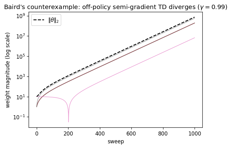
Replacing the value table with a parametric approximator: linear value functions, semi-gradient TD, and the projected Bellman operator. Why on-policy semi-gradient TD converges to a bounded-error fixed point, and why function approximation, bootstrapping, and off-policy training together can diverge — the deadly triad, witnessed by Baird's counterexample.

Function Approximation and the Deadly Triad

Where we are. Every method so far stored one number per state in a table. That ends the moment the state space is large or continuous: we must approximate the value function with a parametric model $V_\theta$ and let it generalize across states. This chapter is the first where the clean contraction story of Chapters 1–4 breaks. Two results frame it. On-policy, semi-gradient TD still converges — but to a projected fixed point whose error is the representation’s projection error, amplified by $1/(1-\discount)$ : approximation changes the fixed point itself. Off-policy, the same update can diverge. The combination that breaks is named the deadly triad — function approximation, bootstrapping, and off-policy training — and Baird’s counterexample is its sharpest witness.

Chapter 5 — at a glance

Goal. Define linear value-function approximation and the semi-gradient TD update; read the TD fixed point as the fixed point of a projected Bellman operator; prove on-policy convergence with a projection-error bound; and see why the deadly triad diverges, on Baird’s counterexample.

Reading time. ~40 minutes; ~65 with the proofs and exercises.

Key insight — the DP bridge. With a table, $\valuefn_\policy$ was the fixed point of a $\discount$ -contraction. With approximation it is replaced by the fixed point of $\Pi\bellman^\policy$ — the Bellman operator followed by a projection back onto the representable subspace. On-policy, that projection is nonexpansive in the right norm and the composition stays a contraction; off-policy, the projection is taken in the wrong norm and the composition can expand. The discount that guaranteed convergence in Chapter 1 is no longer enough on its own.

Linear approximation and semi-gradient TD

Replace the table $V \in \R^{\statespace}$ with a parametric $V_\theta$ . We focus on the linear case, where a feature map $\phi:\statespace\to\R^d$ ( $d \ll \lvert\statespace\rvert$ ) gives

V_\theta(s) = \theta^\top \phi(s), \qquad \theta \in \R^d .

The representable value functions form a $d$ -dimensional subspace $\{\Phi\theta : \theta\in\R^d\}$ of $\R^{\statespace}$ , where $\Phi$ stacks the feature rows. Learning now adjusts $\theta$ , and a value learned at one state moves the values of all states sharing features — generalization, the whole point.

Definition 5.1 (Semi-gradient TD(0)).

Given a transition $(S_t, R_{t+1}, S_{t+1})$ , semi-gradient TD(0) updates

\theta \;\leftarrow\; \theta + \alpha\,\delta_t\,\phi(S_t), \qquad \delta_t = R_{t+1} + \discount\,\theta^\top\phi(S_{t+1}) - \theta^\top\phi(S_t).

It is called semi-gradient because it treats the bootstrap target $\discount\,\theta^\top\phi(S_{t+1})$ as fixed — it does not differentiate the target with respect to $\theta$ , so the update is not the true gradient of any fixed objective.

That last point is the crux of the chapter.

A true-gradient method on a fixed loss cannot diverge to infinity; semi-gradient TD can, because the “target” it descends toward moves with

\theta

The projected Bellman operator

Where does semi-gradient TD converge, when it does? Not to $\bellman^\policy V_\theta$ — that generally leaves the representable subspace and is not expressible as any $\theta$ . The update implicitly projects it back.

Definition 5.2 (Projection and the TD fixed point).

Let $\mu$ be a distribution over states and $\langle x,y\rangle_\mu = \sum_s \mu(s)x(s)y(s)$ the weighted inner product, with norm $\norm{\cdot}_\mu$ . The projection $\Pi_\mu$ maps a value function to the nearest representable one, $\Pi_\mu x = \arg\min_{\theta}\norm{\Phi\theta - x}_\mu$ . The TD fixed point is the $V_\theta$ satisfying

V_\theta = \Pi_\mu\,\bellman^\policy V_\theta ,

the fixed point of the composed projected Bellman operator $\Pi_\mu\bellman^\policy$ .

Semi-gradient TD is a stochastic-approximation scheme (Chapter 4) for this fixed point: in expectation, under the state-visitation distribution $\mu$ its update drives $\theta$ toward $\Pi_\mu\bellman^\policy V_\theta$ . Whether that iteration converges hinges entirely on whether $\Pi_\mu\bellman^\policy$ is a contraction — which depends on $\mu$ .

When it works: on-policy convergence

Proposition 5.1 (On-policy convergence and the projection-error bound).

Let $\mu$ be the on-policy stationary distribution of $\policy$ (so $\mu^\top P_\policy = \mu^\top$ ). Then $\bellman^\policy$ is a $\discount$ -contraction in $\norm{\cdot}_\mu$ , and $\Pi_\mu$ is nonexpansive in $\norm{\cdot}_\mu$ , so $\Pi_\mu\bellman^\policy$ is a $\discount$ -contraction with a unique fixed point $V_{\theta^\star}$ . Its error is the projection error, amplified by the horizon:

\norm{V_{\theta^\star} - \valuefn_\policy}_\mu \;\le\; \frac{1}{1-\discount}\, \norm{\Pi_\mu \valuefn_\policy - \valuefn_\policy}_\mu .

Proof.

Two facts compose. (i) Under the stationary $\mu$ , the transition operator is nonexpansive in $\norm{\cdot}_\mu$ :

\begin{aligned} \norm{P_\policy x}_\mu^2 &= \sum_s \mu(s)\Big(\sum_{s'}P_\policy(s'\mid s)\,x(s')\Big)^2 && \text{(definition)} \\ &\le \sum_s \mu(s)\sum_{s'}P_\policy(s'\mid s)\,x(s')^2 && \text{(Jensen; }P_\policy(\cdot\mid s)\text{ a distribution)} \\ &= \sum_{s'}\Big(\sum_s \mu(s)P_\policy(s'\mid s)\Big)x(s')^2 = \sum_{s'}\mu(s')\,x(s')^2 = \norm{x}_\mu^2 && \text{(}\mu^\top P_\policy = \mu^\top\text{).} \end{aligned}

Since $\bellman^\policy x - \bellman^\policy y = \discount P_\policy(x-y)$ , this gives $\norm{\bellman^\policy x - \bellman^\policy y}_\mu \le \discount\norm{x-y}_\mu$ . (ii) $\Pi_\mu$ is an orthogonal projection in $\langle\cdot,\cdot\rangle_\mu$ , hence nonexpansive. So $\Pi_\mu\bellman^\policy$ is a $\discount$ -contraction and has a unique fixed point $V_{\theta^\star}$ (Banach, Ch. 1). For the bound, since $\bellman^\policy\valuefn_\policy = \valuefn_\policy$ we have $\Pi_\mu\valuefn_\policy = \Pi_\mu\bellman^\policy\valuefn_\policy$ , so

\norm{V_{\theta^\star} - \Pi_\mu\valuefn_\policy}_\mu = \norm{\Pi_\mu\bellman^\policy V_{\theta^\star} - \Pi_\mu\bellman^\policy\valuefn_\policy}_\mu \le \discount\norm{V_{\theta^\star} - \valuefn_\policy}_\mu .

With the triangle inequality $\norm{V_{\theta^\star}-\valuefn_\policy}_\mu \le \norm{V_{\theta^\star}-\Pi_\mu\valuefn_\policy}_\mu + \norm{\Pi_\mu\valuefn_\policy - \valuefn_\policy}_\mu$ , substitute and solve to get the stated bound. $\qquad\blacksquare$

Two readings. First, convergence is conditional: it rests on $\mu$ being the on-policy distribution, the one fact that makes $P_\policy$ nonexpansive.

Second, the fixed point moved: even at convergence the error is the projection error

\norm{\Pi_\mu\valuefn_\policy - \valuefn_\policy}_\mu

— what the feature space cannot represent — blown up by

1/(1-\discount)

. With a table the projection error is zero and we recover

\valuefn_\policy

exactly; with a poor feature space the fixed point can be far from

\valuefn_\policy

. Tsitsiklis and Van Roy Tsitsiklis & Van Roy (1997) established exactly this convergence and bound for on-policy linear TD.

The deadly triad

Proposition 5.1 needed all three of its ingredients to be benign. Drop the on-policy assumption and the guarantee collapses. The instability requires the conjunction of three elements, each harmless alone — the deadly triad Sutton & Barto (2018) :

Function approximation — a value model with fewer parameters than states.
Bootstrapping — TD/DP targets that reuse current estimates (vs. Monte Carlo’s full returns).
Off-policy training — updating from a distribution other than the policy’s own.

Any two are safe: tabular off-policy bootstrapping is Q-learning (Chapter 4, convergent); on-policy bootstrapping with approximation is Proposition 5.1; Monte Carlo with approximation and off-policy data is a genuine gradient method and is stable. All three together can make $\Pi_\mu\bellman^\policy$ — now with $\mu$ the wrong (off-policy) distribution — an expansion, and the parameters diverge to infinity. Baird Baird (1995) built the canonical witness.

Example 5.1 (Baird's counterexample).

Seven states, a linear feature map of dimension eight, and zero reward everywhere — so $\valuefn_\policy = 0$ is trivially representable ( $\theta = 0$ ). The target policy always takes the “solid” action (to the seventh state); the behaviour policy explores all states (off-policy). Off-policy semi-gradient TD with uniform state weighting applies a linear update $\theta_{k+1} = (I + \alpha A)\theta_k$ whose matrix $A$ has an eigenvalue with positive real part. The weights diverge geometrically even though a perfect, zero-error solution sits at the origin.

Eight weight trajectories all growing in magnitude without bound over sweeps, on a log-scaled vertical axis. — Off-policy semi-gradient TD on Baird's counterexample (gamma = 0.99): every component of the linear weight vector diverges, and the value-error norm grows without bound, although the exact solution theta = 0 has zero error. Produced by experiments/python/week05/baird.py.

The lesson is not that approximation is hopeless but that the interaction is what bites: the projected operator’s contraction was an on-policy privilege, and off-policy data revokes it. The next chapter’s engineering — target networks and replay — exists precisely to tame this instability well enough to train deep off-policy value functions in practice.

Beyond semi-gradient: LSTD and true-gradient methods

Two routes around the difficulty are worth naming. Least-squares TD (LSTD) solves the linear TD fixed-point equations directly: accumulate $A = \sum_t \phi(S_t)\big( \phi(S_t) - \discount\phi(S_{t+1})\big)^\top$ and $b = \sum_t \phi(S_t)R_{t+1}$ , then set $\theta^\star = A^{-1}b$ — no step size, far more sample-efficient per datum, converging to the same on-policy fixed point as Proposition 5.1. Gradient-TD methods (GTD, TDC) instead descend a true objective (the projected Bellman error), restoring convergence even off-policy at the cost of a second set of weights. Both are the subject of the roadmap’s extension; LSTD appears in the companion.

The dynamic-programming bridge

Function approximation is the first crack in the contraction spine. Chapters 1–4 chased the unique fixed point of a $\discount$ -contraction; here the object becomes $\Pi_\mu\bellman^\policy$ , and its fixed point both moves (by the projection error) and, off-policy, may not exist as a stable limit at all. Two bridges forward:

To control (LQR, Ch. 13). The linear-quadratic regulator is the lucky case where the optimal value is exactly quadratic — representable with zero projection error — so the approximation never bites and the Riccati recursion converges cleanly. Most of control’s tractable cases are exactly this: a function class the true value lives inside.
To deep RL (Week 6). DQN keeps bootstrapping, off-policy data, and a (nonlinear) approximator — the full triad — and survives by engineering the instability down: a slowly-updated target network freezes the bootstrap target, and experience replay decorrelates and re-weights the update distribution toward something tamer.

What’s next

Week 6 builds DQN: the replay buffer and target network as direct countermeasures to the deadly triad, scaling approximate value learning to pixels.

Exercises

(Derive) Write the semi-gradient TD(0) update for linear $V_\theta$ and show it is not the gradient of $\tfrac12\E[\delta_t^2]$ . Identify the missing term.

Solution
$\nabla_\theta\tfrac12\delta_t^2 = \delta_t\nabla_\theta\delta_t = \delta_t\big( \discount\phi(S_{t+1}) - \phi(S_t)\big)$ . Semi-gradient TD uses $-\delta_t\phi(S_t)$ (ascending $\delta_t\phi(S_t)$ ), dropping the $\discount\delta_t\phi(S_{t+1})$ term from differentiating the target. The dropped term is exactly what would make it a true gradient — and what, when present (residual-gradient methods), changes the fixed point and the stability.
(Prove) Show $\Pi_\mu\bellman^\policy$ is a $\discount$ -contraction in $\norm{\cdot}_\mu$ when $\mu$ is the on-policy distribution, and derive the projection-error bound (Prop. 5.1).

Solution
$\bellman^\policy$ is a $\discount$ -contraction in $\norm{\cdot}_\mu$ because $P_\policy$ is nonexpansive under the stationary $\mu$ (Jensen + $\mu^\top P_\policy = \mu^\top$ ); $\Pi_\mu$ is nonexpansive as an orthogonal projection; the composition is a $\discount$ -contraction. The bound follows from $\Pi_\mu\valuefn_\policy = \Pi_\mu\bellman^\policy\valuefn_\policy$ and the triangle inequality, as in the proof above.
(Compute) In Baird’s setup the update is $\theta_{k+1} = (I + \alpha A)\theta_k$ . What property of $A$ (or of $I + \alpha A$ ) causes divergence, and why does a small $\alpha$ not prevent it?

Solution
Divergence occurs iff $I + \alpha A$ has spectral radius $> 1$ , i.e. $A$ has an eigenvalue with positive real part (for small $\alpha>0$ , $\rho(I+\alpha A)>1$ exactly then). Shrinking $\alpha$ only slows the geometric blow-up; it cannot flip the sign of the unstable eigenvalue. The companion computes $A$ ‘s spectrum.
(Implement) Verify on the companion that on-policy semi-gradient TD converges to (near) $\valuefn_\policy$ on the random walk, while off-policy semi-gradient TD on Baird’s counterexample diverges (the committed figure).

Solution
See experiments/python/week05/test_fa.py: on-policy semi-gradient TD with tabular-complete features matches dp.policy_evaluation within a sampling tolerance and keeps bounded weights; Baird’s off-policy update grows the weight norm without bound (the divergence the figure plots).
(Extend) Implement LSTD and confirm it recovers the same on-policy fixed point as semi-gradient TD (and $\valuefn_\policy$ exactly when the features are tabular-complete).

Solution
LSTD solves $A\theta = b$ with $A = \sum_t\phi(S_t)(\phi(S_t)-\discount\phi(S_{t+1}))^\top$ , $b=\sum_t\phi(S_t)R_{t+1}$ ; its solution is the TD fixed point. With tabular-complete features the projection error is zero and $\theta^\star$ reproduces $\valuefn_\policy$ , which the companion’s lstd asserts against the Week-1 linear solve.

Companion code

The Week-5 companion lives at experiments/python/week05/ and reuses the Week-3 random walk and the Week-1 dp.policy_evaluation oracle. It is the chapter’s two poles side by side: a convergent on-policy method and a divergent off-policy one. (The roadmap suggests tile coding on MountainCar-v0; the random walk is used here because it has a closed-form $\valuefn_\policy$ to test against — MountainCar tile-coding is a natural deferred showcase that lacks an exact oracle.)

fa.py — linear semi_gradient_td (constant step size with Polyak–Ruppert averaging) and lstd for a generic (P, R, policy) with an arbitrary feature matrix $\Phi$ . Pure NumPy.
baird.py — Baird’s seven-state counterexample: builds the feature matrix and the off-policy expected-update matrix $A$ , iterates to divergence, and (with --plot) renders the committed divergence figure.
test_fa.py — mathematical-correctness tests: on-policy semi-gradient TD converges to the analytic $\valuefn_\policy$ (and stays bounded); LSTD recovers $\valuefn_\policy$ with tabular-complete features; and Baird’s off-policy update diverges (the weight norm grows without bound while $A$ has an unstable eigenvalue).

# core algorithms + correctness tests (pure NumPy, no Gymnasium needed)
PYTHONPATH=. pytest experiments/python/week05/test_fa.py -q

# regenerate the committed Baird divergence figure
PYTHONPATH=. python experiments/python/week05/baird.py --plot

Part I · Foundations Week 6 Published dqn.py test_dqn.py

The DQN Family

Making approximate Q-learning stable enough for pixels: experience replay and target networks as direct countermeasures to the deadly triad, the overestimation bias that motivates Double DQN, and the dueling, prioritized, and Rainbow refinements. The engineering that scaled value-based RL to Atari.

The DQN Family

Where we are. Chapter 4 gave us Q-learning; Chapter 5 warned that combining bootstrapping, off-policy data, and function approximation — the deadly triad — can diverge. The deep Q-network is that exact combination (Q-learning, off-policy, with a neural-network approximator), and naively it does diverge. What made it work on Atari from pixels — first as a 2013 workshop result Mnih et al. (2013) , then at human level Mnih et al. (2015) — was not new theory but two pieces of engineering that tame the triad’s two instabilities: experience replay and a target network. This chapter is about that engineering — and the overestimation bias that the next refinement, Double DQN, corrects.

Chapter 6 — at a glance

Goal. Write the DQN loss as a semi-gradient regression; understand experience replay and target networks as countermeasures to the deadly triad’s two failure modes; prove the max-operator overestimation bias and read Double DQN off it; and place dueling, prioritized replay, and Rainbow.

Reading time. ~35 minutes; ~55 with the companion and exercises.

Key insight — the DP bridge. DQN keeps the Bellman optimality backup of Chapter 1 as its regression target, but the deadly triad (Chapter 5) means that target both moves (it depends on the weights being trained) and is fed correlated, off-policy data. Replay re-weights and decorrelates the data; the target network freezes the backup operator for a stretch, turning a moving-target chase into a sequence of stationary supervised problems. Neither restores a true contraction — they buy enough stability for gradient descent to win in practice.

From Q-learning to a deep Q-network

Replace the Q-table with a network $Q_\theta(s,a)$ and fit it to the sampled Bellman optimality target. DQN minimizes, over transitions $(s,a,r,s')$ drawn from a replay buffer $\mathcal{D}$ ,

L(\theta) = \E_{(s,a,r,s')\sim\mathcal{D}}\Big[\big(\, r + \discount \max_{a'} Q_{\theta^-}(s',a') - Q_\theta(s,a)\,\big)^2\Big],

where $\theta^-$ are the target-network weights. As in Chapter 5 this is a semi-gradient method: we differentiate only $Q_\theta(s,a)$ , treating the target as fixed. Two structural problems would sink naive online training, and DQN answers each:

Correlated data. Consecutive transitions in a trajectory are highly correlated, violating the i.i.d. assumption gradient descent leans on.
A moving target. The regression target uses the same network being updated, so every gradient step shifts the target it was chasing — the bootstrap instability of the triad.

Experience replay

The first fix stores each transition $(s,a,r,s')$ in a fixed-capacity buffer $\mathcal{D}$ and trains on uniformly sampled minibatches rather than the latest transition. Three benefits follow: sampling across many past episodes decorrelates the minibatch toward the i.i.d. regime; each transition is reused many times, improving sample efficiency; and the update distribution becomes the buffer’s mixture rather than the current policy’s trajectory, re-weighting away from the pathological off-policy distributions that drive divergence.

The idea is old — it is the model-free, sampled descendant of the prioritized sweeping of Chapter 2 — and its prioritized variant returns shortly.

Target networks

The second fix freezes the bootstrap. DQN keeps a separate copy $Q_{\theta^-}$ of the network, holds it fixed while training $Q_\theta$ , and refreshes $\theta^- \leftarrow \theta$ only every $C$ steps (a hard update) or by a slow Polyak average $\theta^- \leftarrow \tau\theta + (1-\tau)\theta^-$ (a soft update). Between refreshes the target $r + \discount\max_{a'}Q_{\theta^-}(s',a')$ is a fixed function, so each interval is an ordinary supervised regression toward a stationary target — exactly the stability the moving-target triad destroyed.

The slower

\theta^-

moves, the more stable and the slower the learning — the central DQN tuning trade-off.

Overestimation and Double DQN

One bias survives even with replay and a target network: the $\max$ in the target overestimates. Because the network’s action-values are noisy estimates, taking their maximum is systematically too high.

Proposition 6.1 (The max overestimates).

Let $\widehat{Q}(s',\cdot)$ be unbiased estimates of the true values $q(s',\cdot)$ , i.e. $\E[\widehat{Q}(s',a)] = q(s',a)$ for each $a$ . Then

\E\big[\max_{a}\widehat{Q}(s',a)\big] \;\ge\; \max_{a}\E\big[\widehat{Q}(s',a)\big] = \max_a q(s',a),

with strict inequality whenever two or more actions’ estimates have positive-variance overlap. The bootstrap target therefore inherits a positive bias.

Proof.

The function $x \mapsto \max_a x_a$ is convex (a pointwise maximum of linear maps). Jensen’s inequality for a convex function gives $\E[\max_a \widehat{Q}(s',a)] \ge \max_a \E[\widehat{Q}(s',a)]$ , and the right side is $\max_a q(s',a)$ by unbiasedness. Jensen is an equality only where the convex function is affine along the distribution’s support; the $\max$ has a kink exactly where the maximizing action changes, so any noise that makes the $\arg\max$ random makes the inequality strict. $\qquad\blacksquare$

Double DQN Hasselt et al. (2016) removes most of this bias by decoupling action selection from evaluation: pick the next action with the online network but evaluate it with the target network,

y^{\text{Double}} = r + \discount\, Q_{\theta^-}\!\big(s',\, \argmax_{a'} Q_\theta(s',a')\big).

The selecting and evaluating estimates now have independent errors, so they no longer conspire to inflate the maximum — a one-line change that measurably improves scores.

Dueling, prioritized replay, and Rainbow

Three further refinements round out the family. The dueling architecture Wang et al. (2016) splits the network into a state-value stream $V(s)$ and an advantage stream $A(s,a)$ , recombined as $Q(s,a) = V(s) + \big(A(s,a) - \tfrac{1}{\lvert\actionspace\rvert}\sum_{a'}A(s,a')\big)$ , so the agent can learn a state is good without estimating every action precisely. Prioritized experience replay Schaul et al. (2016) samples transitions in proportion to their Bellman-residual magnitude — Chapter 2’s prioritized sweeping, now over replayed transitions — with importance weights to correct the sampling bias. Rainbow Hessel et al. (2018) combines six such improvements (double, dueling, prioritized replay, multi-step returns, distributional values, and noisy exploration) and ablates each, showing they are largely complementary.

From states to pixels

DQN’s headline result was learning from raw Atari frames on the Arcade Learning Environment Bellemare et al. (2013) . The pixel pipeline adds its own engineering: grayscale and downsample each frame, stack four frames so velocity is observable (a single frame is not Markov), skip frames, clip rewards to $\{-1,0,+1\}$ , and read the stack with a convolutional network. None of this changes the algorithm — it changes the features the same loss is regressed on.

Reliable comparison across all this machinery is itself hard — reproducibility studies and standardized implementations Raffin et al. (2021) exist precisely because small details swing results, a theme Week 8 returns to.

The dynamic-programming bridge

DQN is the deadly triad (Chapter 5) survived by engineering rather than dissolved by theory. The regression target is still the sampled Bellman optimality backup of Chapter 1; the two additions each blunt one edge of the triad. Replay re-weights and decorrelates the update distribution — the off-policy edge — and is the model-free heir to prioritized sweeping (Chapter 2). The target network freezes the bootstrap operator for $C$ steps — the moving-target edge — converting divergent fixed-point chasing into a sequence of stationary regressions. The discount $\discount$ that guaranteed convergence with a table now only bounds the per-interval target; stability is bought, not proved.

What’s next

Week 7 changes the object of optimization entirely: instead of learning values and acting greedily, policy-gradient methods parameterize and optimize the policy directly, sidestepping the $\max$ and its overestimation, and extending naturally to continuous actions.

Exercises

(Prove) Show $\E[\max_a \widehat{Q}(s',a)] \ge \max_a q(s',a)$ for unbiased $\widehat{Q}$ , and state when the inequality is strict (Prop. 6.1).

Solution
$\max_a$ is convex, so Jensen gives $\E[\max_a\widehat{Q}(s',a)] \ge \max_a\E[\widehat{Q}(s',a)] = \max_a q(s',a)$ . It is strict whenever the noise makes the $\arg\max$ random (two actions’ estimates overlap with positive probability), because the $\max$ is non-affine across the kink where the maximizer switches.
(Derive) Write the Double DQN target and explain why it reduces the overestimation of Proposition 6.1.

Solution
$y^{\text{Double}} = r + \discount Q_{\theta^-}(s', \argmax_{a'}Q_\theta(s',a'))$ . Selection uses $Q_\theta$ , evaluation uses $Q_{\theta^-}$ ; their estimation errors are (largely) independent, so the action chosen as best by one network is not automatically assigned an inflated value by the same network. The $\E[\max]$ bias becomes the much smaller bias of evaluating a possibly-suboptimal action.
(Compute) A replay buffer of capacity 3 receives transitions $t_1,\dots,t_5$ in order. Which are stored after $t_5$ , and why does a hard target update at step $C$ leave $\theta^-$ momentarily equal to $\theta$ ?

Solution
A circular buffer of capacity 3 keeps the three most recent, $\{t_3,t_4,t_5\}$ ( $t_1,t_2$ overwritten). A hard update copies $\theta^- \leftarrow \theta$ , so immediately after step $C$ the two networks are identical; they diverge again as $\theta$ updates over the next $C$ steps while $\theta^-$ is held fixed.
(Implement) In the companion, verify the replay buffer, target-update, and TD-target components, and that DQN learns CartPole well above the random-return baseline within a fixed step budget.

Solution
See experiments/python/week06/test_dqn.py: circular-buffer overwrite and sample shapes; hard/soft target updates; the done-masked TD target and the Double-DQN selection/evaluation split; the empirical overestimation of the plain max; and a seeded CartPole run whose mean return rises far above the ~22 random baseline.
(Extend) Add Double and Dueling variants and measure the overestimation gap (the plain-max target minus the Double target) over training.

Solution
The companion exposes double and dueling flags; the plain-max target sits above the Double target early in training (when value estimates are noisiest) and the gap shrinks as the network sharpens — the empirical face of Proposition 6.1.

Companion code

The Week-6 companion lives at experiments/python/week06/ and is the chapter’s first PyTorch code. Its correctness suite follows the repo’s deep-RL convention: fast, deterministic component tests for the pieces, plus a seeded simple-environment convergence check — heavy pixel environments are a deferred @slow showcase, not a graded test, in line with the 8 GB GPU budget.

dqn.py — a minimal DQN on CartPole-v1: a circular ReplayBuffer, an MLP QNetwork (and a DuelingQNetwork), an exposed td_target (plain and Double), hard/soft target updates, and the training loop, with double/dueling flags.
test_dqn.py — component-correctness tests (replay overwrite + sample shapes; target-network hard/soft updates; the done-masked Bellman target; the Double-DQN selection/evaluation split; the max-overestimation of Prop. 6.1) plus a seeded CartPole run asserting the mean return clears the random baseline by a wide margin.

# component tests + a seeded CartPole learning check (PyTorch; ~1-2 min on CPU)
PYTHONPATH=. pytest experiments/python/week06/test_dqn.py -q

# worked CartPole training run (prints the learning curve summary)
PYTHONPATH=. python experiments/python/week06/dqn.py --double --episodes 400

Part I · Foundations Week 7 Published reinforce.py test_reinforce.py

Policy Gradient Foundations

Optimizing a parameterized stochastic policy directly by gradient ascent on expected return: the policy gradient theorem via the log-derivative trick, REINFORCE, and baselines as variance-reducing control variates. Policy gradients as Monte Carlo sensitivity analysis — and the advantage that bridges to actor-critic.

Policy Gradient Foundations

Where we are. Every method so far learned a value and acted greedily — the $\argmax$ of Chapters 4–6. Policy-gradient methods discard that indirection: they parameterize the policy $\policy_\theta(a\mid s)$ and ascend the gradient of expected return directly. This sidesteps the $\max$ and its overestimation (Chapter 6), handles stochastic policies and continuous actions natively, and rests on one identity — the log-derivative trick — that turns “differentiate an expectation you can only sample” into “weight samples by the score $\nabla_\theta\log\policy_\theta$ .” The roadmap’s framing is exact: policy gradients are Monte Carlo sensitivity analysis.

Chapter 7 — at a glance

Goal. State the objective $J(\theta)$ ; prove the policy gradient theorem with the log-derivative trick; read REINFORCE off it; prove a state-dependent baseline leaves the gradient unbiased while cutting variance; and identify the advantage as the variance-minimizing weight.

Reading time. ~35 minutes; ~55 with the proofs and exercises.

Key insight — the DP bridge. Value-based RL solved the Bellman fixed point and derived a policy by $\argmax$ . Policy gradients optimize the policy as the primal object and let value functions return only as a baseline/critic (Week 8). The weight that minimizes the estimator’s variance is the advantage $\advantage = \qfn - \valuefn$ — the same advantage that drives actor-critic and that, in continuous time, is the adjoint/Hamiltonian sensitivity of optimal control (Part II).

The objective and the score

Let the policy be $\policy_\theta(a\mid s)$ , differentiable in $\theta$ . A trajectory $\tau = (S_0, A_0, R_1, \dots)$ has return $\return(\tau) = \sum_{t\ge 0}\discount^t R_{t+1}$ , and the objective is its expectation,

J(\theta) \defeq \E_{\tau\sim\policy_\theta}\!\big[\,\return(\tau)\,\big].

We cannot differentiate $J$ by differentiating the reward — the dependence on $\theta$ is through the sampling distribution of $\tau$ , not the integrand. The score function $\nabla_\theta\log\policy_\theta(a\mid s)$ is what carries that dependence, via one identity.

The policy gradient theorem

The gradient of $J$ has a famously clean form, due to Sutton et al. Sutton et al. (2000) : an expectation of the score weighted by the action-value, with no derivative of the unknown dynamics anywhere in it.

Theorem 7.1 (Policy gradient theorem).

The gradient of the expected return is

\nabla_\theta J(\theta) = \E_{\tau\sim\policy_\theta}\!\Big[\, \return(\tau)\sum_{t\ge 0}\nabla_\theta\log\policy_\theta(A_t\mid S_t)\,\Big] = \E_{\policy_\theta}\!\Big[\sum_{t\ge 0}\nabla_\theta\log\policy_\theta(A_t\mid S_t)\,\qfn_{\policy_\theta}(S_t,A_t)\Big].

No derivative of the dynamics or the reward appears — only the score of the policy.

Proof.

Write $J(\theta) = \int p_\theta(\tau)\,\return(\tau)\,d\tau$ with trajectory density $p_\theta(\tau) = p(s_0)\prod_t \policy_\theta(a_t\mid s_t)\,\transition(s_{t+1}\mid s_t,a_t)$ . Differentiate and apply the log-derivative trick $\nabla_\theta p_\theta = p_\theta\nabla_\theta\log p_\theta$ :

\begin{aligned} \nabla_\theta J &= \int \nabla_\theta p_\theta(\tau)\,\return(\tau)\,d\tau && \text{(differentiate under the integral)} \\ &= \int p_\theta(\tau)\,\nabla_\theta\log p_\theta(\tau)\,\return(\tau)\,d\tau && \text{(log-derivative trick)} \\ &= \E_{\tau}\!\big[\,\return(\tau)\,\nabla_\theta\log p_\theta(\tau)\,\big] && \text{(definition of expectation).} \end{aligned}

In $\log p_\theta(\tau) = \log p(s_0) + \sum_t\big[\log\policy_\theta(a_t\mid s_t) + \log\transition(s_{t+1}\mid s_t,a_t)\big]$ the initial-state and dynamics terms do not depend on $\theta$ , so $\nabla_\theta\log p_\theta(\tau) = \sum_t\nabla_\theta\log \policy_\theta(a_t\mid s_t)$ — the model need not be known or differentiated. That gives the first form. Using causality (an action cannot influence past rewards, $\E[\nabla_\theta\log\policy_\theta(A_t\mid S_t)R_{t'}] = 0$ for $t' \le t$ ) replaces $\return(\tau)$ by the return-to-go, whose conditional expectation is $\qfn_{\policy_\theta}(S_t,A_t)$ , giving the second. $\qquad\blacksquare$

The estimator is Monte Carlo sensitivity analysis: it estimates $\nabla_\theta\E[ \cdot]$ from samples without differentiating the sampled function, by reweighting each sample by its score.

It is unbiased and, being Monte Carlo (Chapter 3), high-variance — which the rest of the chapter attacks.

REINFORCE

Sampling the theorem’s expectation gives the REINFORCE algorithm Williams (1992) : roll out episodes under $\policy_\theta$ , form the returns-to-go $\return_t$ , and ascend

\widehat{\nabla_\theta J} = \sum_t \nabla_\theta\log\policy_\theta(A_t\mid S_t)\,\return_t, \qquad \theta \leftarrow \theta + \alpha\,\widehat{\nabla_\theta J}.

It is unbiased and model-free, the policy-space counterpart of Monte Carlo value estimation — and inherits Monte Carlo’s variance.

The single most effective fix is a baseline.

Baselines as control variates

Proposition 7.1 (A state baseline is unbiased).

For any function $b(s)$ that does not depend on the action,

\E_{\policy_\theta}\!\big[\,\nabla_\theta\log\policy_\theta(A_t\mid S_t)\,b(S_t)\,\big] = 0,

so subtracting $b(S_t)$ from the return weight in the policy gradient leaves it unbiased, while choosing $b$ to track the typical return reduces its variance.

Proof.

Condition on $S_t = s$ and average the score over actions:

\E_{a\sim\policy_\theta(\cdot\mid s)}\!\big[\nabla_\theta\log\policy_\theta(a\mid s)\big] = \sum_a \policy_\theta(a\mid s)\,\frac{\nabla_\theta\policy_\theta(a\mid s)}{\policy_\theta(a\mid s)} = \sum_a \nabla_\theta\policy_\theta(a\mid s) = \nabla_\theta\sum_a\policy_\theta(a\mid s) = \nabla_\theta 1 = 0.

Hence $\E[\nabla_\theta\log\policy_\theta(A_t\mid S_t)\,b(S_t)] = \E[b(S_t)\cdot 0] = 0$ : subtracting $b(S_t)$ changes the gradient’s variance but not its mean. The variance-minimizing choice makes the weight a centered quantity; taking $b(s) = \valuefn_{\policy_\theta}(s)$ turns the weight into the advantage $\advantage(s,a) = \qfn(s,a) - \valuefn(s)$ . $\qquad\blacksquare$

A baseline is precisely a control variate: a zero-mean term subtracted to shrink variance without moving the estimate.

With

b = \valuefn

, the policy gradient becomes

\E[\sum_t \nabla_\theta\log\policy_\theta(A_t\mid S_t)\,\advantage(S_t,A_t)]

— the form every actor-critic method (Week 8) estimates. Learning the baseline

\valuefn

is what makes it a critic.

The dynamic-programming bridge

Policy gradients invert the value-based pattern. Chapters 4–6 solved a Bellman fixed point and read off a greedy policy; here the policy is the primal object optimized by gradient ascent, and value functions re-enter only as the baseline/critic that tames variance. Three threads carry forward:

To actor-critic (Week 8). Learn $\valuefn$ (or the advantage directly) as the baseline; the policy is the actor, the value the critic. Generalized advantage estimation tunes the bias–variance of $\advantage$ , and trust regions (PPO/TRPO) control the ascent step size in policy space.
To continuous control (Week 9). No $\argmax$ over actions is ever taken, so continuous action spaces are immediate — the setting where DDPG, TD3, and SAC live.
To optimal control (Part II). Differentiating an expected cost through the dynamics is the discrete, stochastic cousin of the adjoint/Hamiltonian sensitivity of Pontryagin’s principle — direct policy search is trajectory optimization with the model replaced by samples.

What’s next

Week 8 learns the baseline as a critic (actor-critic), tunes the advantage with generalized advantage estimation, and adds trust regions (TRPO/PPO) to bound the policy update — turning REINFORCE’s noisy ascent into a stable, sample-reusing optimizer.

Exercises

(Derive) Derive the policy gradient theorem from $J(\theta) = \E_{\tau}[\return(\tau)]$ using the log-derivative trick, and show the dynamics terms drop (Theorem 7.1).

Solution
$\nabla_\theta J = \int\nabla_\theta p_\theta(\tau)\return(\tau)d\tau = \E_\tau[ \return(\tau)\nabla_\theta\log p_\theta(\tau)]$ . Since $\log p_\theta(\tau)$ splits into initial-state, policy, and dynamics terms and only the policy terms carry $\theta$ , $\nabla_\theta\log p_\theta(\tau) = \sum_t\nabla_\theta\log\policy_\theta(a_t \mid s_t)$ — the model cancels.
(Prove) Show a state-dependent baseline $b(s)$ leaves the policy gradient unbiased, i.e. $\E[\nabla_\theta\log\policy_\theta(A\mid S)\,b(S)] = 0$ (Prop. 7.1).

Solution
$\E_{a\sim\policy_\theta(\cdot\mid s)}[\nabla_\theta\log\policy_\theta(a\mid s)] = \sum_a\nabla_\theta\policy_\theta(a\mid s) = \nabla_\theta\sum_a\policy_\theta(a\mid s) = \nabla_\theta 1 = 0$ . Multiplying by $b(s)$ (constant in $a$ ) and taking the outer expectation over $S$ preserves the zero.
(Compute) For a softmax policy $\policy_\theta(a\mid s) \propto \exp(\theta_a^\top\phi(s))$ , compute the score $\nabla_{\theta_j}\log\policy_\theta(a \mid s)$ .

Solution
$\nabla_{\theta_j}\log\policy_\theta(a\mid s) = \big(\mathbf{1}[j=a] - \policy_\theta(j\mid s)\big)\phi(s)$ — the feature, weighted by “taken minus probability.” Summed over $a\sim\policy_\theta$ this is zero (Prop. 7.1), the discrete face of the expected-score identity.
(Implement) In the companion, verify the returns-to-go computation, that the expected score is zero (the baseline mechanism), that a baseline reduces gradient variance without bias, and that REINFORCE learns CartPole above the random baseline.

Solution
See experiments/python/week07/test_reinforce.py: a hand-checked discounted return-to-go; $\sum_a\policy(a\mid s)\nabla_\theta\log\policy(a\mid s)\approx 0$ for a softmax network; a bandit where the baselined estimator has strictly lower variance; and a seeded CartPole run whose mean return clears the ~22 random baseline.
(Extend) Add an entropy bonus $\beta\,\mathcal{H}(\policy_\theta(\cdot\mid s))$ to the objective and explain its effect on exploration. (The roadmap’s JAX jax.grad variant is deferred to the dedicated JAX track.)

Solution
The entropy bonus rewards less-peaked policies, slowing premature convergence to a deterministic policy and sustaining exploration; its gradient adds $\beta\nabla_\theta \mathcal{H}$ , pushing toward higher-entropy distributions. It reappears, promoted from a bonus to the objective, in maximum-entropy RL (Week 9, SAC).

Companion code

The Week-7 companion lives at experiments/python/week07/ and is PyTorch REINFORCE on CartPole-v1, with and without a value baseline.

reinforce.py — a softmax PolicyNetwork, the discounted compute_returns (returns-to-go), and a REINFORCE training loop with an optional learned-value baseline and return normalization.
test_reinforce.py — component-correctness tests (hand-checked returns-to-go; the expected score $\sum_a\policy\,\nabla\log\policy = 0$ that underlies Prop. 7.1; a bandit where the baselined gradient estimator has strictly lower variance) plus a seeded CartPole run learning well above the random-return baseline.

# component tests + a seeded CartPole learning check (PyTorch; ~1-2 min on CPU)
PYTHONPATH=. pytest experiments/python/week07/test_reinforce.py -q

# worked REINFORCE training run (with the value baseline)
PYTHONPATH=. python experiments/python/week07/reinforce.py --baseline --episodes 800

Part I · Foundations Week 8 Published ppo.py test_ppo.py

Actor-Critic, GAE, PPO, and TRPO

Turning REINFORCE into a stable, sample-reusing optimizer: actor-critic with a learned baseline, generalized advantage estimation as a bias–variance dial, and trust regions (TRPO/PPO) as step-size control in policy space. Why the clipped surrogate works, and why implementation details decide the score.

Actor-Critic, GAE, PPO, and TRPO

Where we are. REINFORCE (Chapter 7) was unbiased but high-variance and strictly on-policy: one noisy gradient step per batch of fresh trajectories, then throw the data away. This chapter turns it into the workhorse of modern on-policy RL by adding three things: a learned critic as the baseline (actor-critic), generalized advantage estimation to tune the advantage’s bias–variance, and a trust region (TRPO/PPO) that bounds how far each update moves the policy — which is what finally lets a batch be reused for several epochs. The roadmap’s framing is the through-line: trust regions are step-size control in policy space.

Chapter 8 — at a glance

Goal. Build actor-critic from Chapter 7’s advantage; derive the GAE recursion and its bias–variance dial; understand TRPO’s constrained step and PPO’s clipped surrogate as two ways to bound the policy update; and see why implementation details dominate reported performance.

Reading time. ~35 minutes; ~55 with the proof and exercises.

Key insight — the DP bridge. Actor-critic is generalized policy iteration (Chapter 1) with approximation: the critic is approximate policy evaluation, the gradient actor is approximate improvement. Policy iteration took the full greedy jump; here improvement is a small, trust-region-controlled step, because the advantage estimate is only trustworthy near the policy that produced the data. GAE’s $\lambda$ is the same bias–variance dial as $n$ -step TD (Chapter 4).

Actor-critic

Chapter 7 ended with the advantage form of the policy gradient, $\nabla_\theta J = \E[\sum_t \nabla_\theta\log\policy_\theta(A_t\mid S_t)\,\advantage(S_t,A_t)]$ . Actor-critic makes the baseline a learned function: an actor $\policy_\theta$ and a critic $\valuefn_\phi$ trained to predict returns, with the advantage estimated from the critic.

Advantage actor-critic (A2C) updates both together — the critic by regressing

\valuefn_\phi

toward the returns, the actor by ascending the score weighted by the critic’s advantage. Konda and Tsitsiklis Konda & Tsitsiklis (2000) established the two-timescale convergence of actor-critic with a linear critic; the critic plays the role of approximate policy evaluation in a sampled, function-approximated generalized policy iteration.

Generalized advantage estimation

How should the advantage be estimated? The one-step TD residual $\delta_t = R_{t+1} + \discount\valuefn_\phi(S_{t+1}) - \valuefn_\phi(S_t)$ is itself a low-variance, high-bias advantage estimate; the full Monte Carlo advantage $\return_t - \valuefn_\phi(S_t)$ is the reverse. Generalized advantage estimation Schulman et al. (2016) interpolates with an exponential weighting.

Proposition 8.1 (The GAE recursion).

The generalized advantage estimator

\advantage^{\text{GAE}(\discount,\lambda)}_t \defeq \sum_{l\ge 0}(\discount\lambda)^l\,\delta_{t+l}

satisfies the backward recursion

\advantage^{\text{GAE}}_t = \delta_t + \discount\lambda\,\advantage^{\text{GAE}}_{t+1}.

Its endpoints are $\lambda=0$ , giving $\advantage_t=\delta_t$ (low variance, high bias), and $\lambda=1$ , giving $\advantage_t=\sum_{l\ge0}\discount^l\delta_{t+l}=\return_t-\valuefn_\phi(S_t)$ (the Monte Carlo advantage: high variance, low bias).

Proof.

Split the defining sum at its first term:

\sum_{l\ge 0}(\discount\lambda)^l\delta_{t+l} = \delta_t + \sum_{l\ge 1}(\discount\lambda)^l\delta_{t+l} = \delta_t + \discount\lambda\sum_{l\ge 0}(\discount\lambda)^l\delta_{t+1+l} = \delta_t + \discount\lambda\,\advantage^{\text{GAE}}_{t+1}.

For $\lambda=1$ , $\sum_{l\ge0}\discount^l\delta_{t+l}$ telescopes: writing $\delta_{t+l} = R_{t+l+1}+\discount\valuefn_\phi(S_{t+l+1})-\valuefn_\phi(S_{t+l})$ , the value terms cancel in pairs, leaving $\sum_{l\ge0}\discount^l R_{t+l+1} - \valuefn_\phi(S_t) = \return_t-\valuefn_\phi(S_t)$ . $\qquad\blacksquare$

The recursion is what the companion computes in one backward pass.

Intermediate

\lambda

(commonly

\approx 0.95

) usually beats both endpoints — the same lesson as

n

-step TD, now applied to the advantage that weights the policy gradient.

Trust regions: TRPO and PPO

REINFORCE and A2C take one gradient step per batch because the advantage estimate is only valid near the policy that generated the data; a large step can collapse performance. The fix is to bound the update — to control the step size in policy space rather than parameter space.

TRPO Schulman et al. (2015) makes this literal: maximize the importance-weighted surrogate $\E[\rho_t\,\advantage_t]$ , with ratio $\rho_t = \policy_\theta(A_t\mid S_t)/\policy_{\text{old}}(A_t\mid S_t)$ , subject to a trust-region constraint $\E[\mathrm{KL}(\policy_{\text{old}}\,\|\,\policy_\theta)] \le \delta$ . The KL ball is the trust region; within it the linearized objective is reliable.

PPO Schulman et al. (2017) replaces the hard constraint with a cheaper clipped surrogate,

L^{\text{CLIP}}(\theta) = \E\big[\min\big(\rho_t\,\advantage_t,\ \mathrm{clip}(\rho_t, 1-\epsilon, 1+\epsilon)\,\advantage_t\big)\big].

The $\min$ makes $L^{\text{CLIP}}$ a pessimistic lower bound on the unclipped surrogate: when an advantage is positive, the objective stops rewarding increases in $\rho_t$ once $\rho_t > 1+\epsilon$ (its gradient there is zero); when negative, it stops once $\rho_t < 1-\epsilon$ .

Either way there is no incentive to push the policy far from

\policy_{\text{old}}

in a single update, so PPO can safely take several epochs of minibatch updates per batch — the sample reuse REINFORCE lacked.

Implementation matters

A sobering empirical fact closes the family. Engstrom et al. Engstrom et al. (2020) showed that much of PPO’s advantage over TRPO comes not from the clipped objective but from code-level details — advantage normalization, value-function clipping, reward scaling, learning-rate annealing, orthogonal initialization — applied alongside it. Together with the broader reproducibility findings of Henderson et al. Henderson et al. (2018) , the lesson is that on-policy deep RL results must be read with the implementation, not just the algorithm, in view. The companion therefore tests the components (the GAE recursion, advantage normalization, the clip) and checks learning on a simple task, rather than chasing a benchmark number.

The dynamic-programming bridge

Actor-critic completes the generalized-policy-iteration picture under approximation. The critic is approximate policy evaluation (Chapter 1’s $\valuefn_\policy$ , learned from samples); the gradient actor is approximate improvement. Where policy iteration took the full greedy jump to $\argmax_a \qfn$ , the actor takes a small step, and the trust region (TRPO’s KL ball, PPO’s clip) is exactly the step-size control that keeps improvement reliable when evaluation is noisy and local. Two bridges:

To continuous control (Week 9). Everything here is on-policy and stochastic; Week 9 turns to off-policy continuous control (DDPG, TD3, SAC), trading sample reuse-by-replay for the on-policy stability bought here by trust regions.
To optimal control (Part II). A trust region on the update is a regularized step — the policy-space analogue of a line search or a Levenberg–Marquardt damping in optimization, and a cousin of MPC’s receding horizon as a bound on how far ahead a single decision commits.

What’s next

Week 9 leaves on-policy methods for off-policy continuous control: the deterministic policy gradient (DDPG), its twin-critic fix (TD3), and maximum-entropy RL (SAC) — where the entropy bonus of Chapter 7 becomes the objective.

Exercises

(Derive) Derive the GAE recursion $\advantage^{\text{GAE}}_t = \delta_t + \discount\lambda\,\advantage^{\text{GAE}}_{t+1}$ from the exponential sum, and show $\lambda=1$ gives the Monte Carlo advantage (Prop. 8.1).

Solution
Split the sum at $l=0$ : $\sum_{l\ge0}(\discount\lambda)^l\delta_{t+l} = \delta_t + \discount\lambda\sum_{l\ge0}(\discount\lambda)^l\delta_{t+1+l} = \delta_t + \discount\lambda\advantage^{\text{GAE}}_{t+1}$ . At $\lambda=1$ the value terms in $\sum_l\discount^l\delta_{t+l}$ telescope to $\return_t-\valuefn_\phi(S_t)$ .
(Prove) Show $L^{\text{CLIP}}$ is a lower bound on the unclipped surrogate $\E[\rho_t\advantage_t]$ , and identify where its gradient with respect to $\rho_t$ is zero.

Solution
$\min(\rho\advantage, \mathrm{clip}(\rho)\advantage) \le \rho\advantage$ pointwise, so the expectation is a lower bound. For $\advantage>0$ the clip caps the term at $(1+\epsilon)\advantage$ once $\rho>1+\epsilon$ , where $\partial/\partial\rho = 0$ ; for $\advantage<0$ it floors at $(1-\epsilon)\advantage$ once $\rho<1-\epsilon$ , again with zero gradient. Inside $[1-\epsilon,1+\epsilon]$ the gradient is $\advantage$ .
(Compute) With $\discount=0.99$ , $\lambda=0.95$ , and TD residuals $\delta = (1.0, 0.5, -0.2)$ at the end of an episode (bootstrap zero), compute $\advantage^{\text{GAE}}$ .

Solution
Backward: $\advantage_2 = -0.2$ ; $\advantage_1 = 0.5 + 0.99\cdot0.95\cdot(-0.2) = 0.3119$ ; $\advantage_0 = 1.0 + 0.99\cdot0.95\cdot0.3119 = 1.2933$ . (The companion’s compute_gae reproduces these.)
(Implement) In the companion, verify the GAE recursion matches the exponential sum and that $\lambda=1$ equals returns minus values; that advantage normalization produces mean-0/unit-variance advantages; that the PPO clip flattens the objective outside $[1-\epsilon,1+\epsilon]$ ; and that PPO learns CartPole above the random baseline.

Solution
See experiments/python/week08/test_ppo.py: compute_gae vs the brute-force $\sum(\discount\lambda)^l\delta$ ; the $\lambda=1$ telescoping identity; the normalization statistics; the clip’s value/gradient outside the range; and a seeded PPO CartPole run clearing the ~22 random baseline.
(Extend) Sweep the PPO clip range $\epsilon$ and add KL early stopping; compare stability across seeds.

Solution
Smaller $\epsilon$ tightens the trust region (more stable, slower); larger loosens it (faster, riskier). KL early stopping halts the epoch loop once the policy has moved a target KL from $\policy_{\text{old}}$ , a direct enforcement of the trust region the clip only approximates — the companion’s --clip/--target-kl flags expose both.

Companion code

The Week-8 companion lives at experiments/python/week08/ and is PyTorch A2C and PPO on CartPole-v1, sharing one actor-critic network.

ppo.py — compute_gae (the backward recursion), an ActorCritic network, the ppo_clip_objective, and a PPO/A2C training loop with advantage normalization and a configurable clip range and epoch count.
test_ppo.py — component-correctness tests (compute_gae vs the closed-form exponential sum; the $\lambda=1$ = returns − values identity; advantage normalization; the PPO clip’s value and zero gradient outside $[1-\epsilon,1+\epsilon]$ ) plus a seeded PPO CartPole run learning above the random baseline.

# component tests + a seeded CartPole learning check (PyTorch; ~1-2 min on CPU)
PYTHONPATH=. pytest experiments/python/week08/test_ppo.py -q

# worked PPO training run on CartPole
PYTHONPATH=. python experiments/python/week08/ppo.py --updates 150

Part I · Foundations Week 9 Published td3.py test_td3.py

Off-Policy Continuous Control: DDPG, TD3, and SAC

Off-policy actor-critic for continuous actions: the deterministic policy gradient (DDPG), the twin-critic overestimation fix (TD3), and maximum-entropy RL (SAC). Why the soft-optimal policy is Boltzmann in the action-value, and how maximum-entropy RL is KL-regularized optimal control — the bridge from learning to Part II.

Off-Policy Continuous Control: DDPG, TD3, and SAC

Where we are. Weeks 7–8 optimized stochastic policies on-policy. This chapter — the last of the RL foundations — turns to off-policy continuous control, where two ideas dominate the model-free baselines. First, the deterministic policy gradient (DDPG) makes continuous actions tractable by pushing the gradient through a differentiable critic instead of sampling them. Second, maximum-entropy RL (SAC) augments the reward with policy entropy, which both stabilizes learning and reveals a deep identity: maximum-entropy RL is KL-regularized optimal control — the bridge out of learning and into Part II. Between them, TD3 fixes the overestimation that Chapter 6 first diagnosed, now arising from the critic’s own bootstrap.

Chapter 9 — at a glance

Goal. State the deterministic policy gradient and read DDPG off it; see how TD3’s twin critics fix overestimation; derive the soft-optimal Boltzmann policy of maximum-entropy RL; and identify maximum-entropy RL with KL-regularized control.

Reading time. ~35 minutes; ~55 with the proofs and exercises.

Key insight — the DP bridge. Continuous actions turn the Bellman backup’s $\max_a$ into an optimization over a continuum: DDPG/TD3 solve it with a gradient actor through the critic; SAC softens it into a $\log\!\sum\exp$ . That soft maximum is exactly the value function of KL-regularized control (Todorov’s linearly-solvable MDPs), and the soft Bellman operator remains a contraction. This is where reinforcement learning and optimal control finally speak the same language — the LQR and MPC of Part II are the model-based, deterministic limit.

The deterministic policy gradient

With a continuous action space the stochastic policy gradient (Chapter 7) must average the score over actions — expensive and high-variance. A deterministic policy $\mu_\theta:\statespace\to\actionspace$ avoids the action integral, and its gradient flows through the critic by the chain rule.

Theorem 9.1 (Deterministic policy gradient).

For a deterministic policy $\mu_\theta$ and its action-value $\qfn_{\mu_\theta}$ , under mild regularity the gradient of the off-policy objective is

\nabla_\theta J(\theta) = \E_{s\sim\rho}\!\Big[\,\nabla_\theta\mu_\theta(s)\,\nabla_a \qfn_{\mu_\theta}(s,a)\big|_{a=\mu_\theta(s)}\Big],

where $\rho$ is the (off-policy) state distribution. The policy is improved by pushing its output up the critic’s action-gradient.

This is the continuous-action analogue of greedy improvement: where a discrete agent takes $\argmax_a \qfn$ , the deterministic actor takes a gradient step in $a$ toward larger $\qfn$ .

Silver et al. Silver et al. (2014) proved the theorem (as the zero-variance limit of the stochastic gradient); Lillicrap et al. Lillicrap et al. (2016) turned it into DDPG — the deterministic actor and critic trained off-policy with the replay buffer and target networks of Chapter 6, and exploration noise added to the actor’s output.

Overestimation returns: TD3

DDPG inherits the deadly-triad fragility and the overestimation bias of Chapter 6 — now produced by the critic bootstrapping on its own optimistic estimates. TD3 Fujimoto et al. (2018) applies three fixes, the first echoing Double DQN:

Twin critics, take the minimum. Train two critics $\qfn_{\phi_1},\qfn_{\phi_2}$ and form the target with $\min(\qfn_{\phi_1},\qfn_{\phi_2})$ — clipped double Q-learning, a continuous cousin of Double DQN that caps the upward bias of Proposition 6.1.
Delayed policy updates. Update the actor (and targets) less often than the critics, so the policy chases a more settled value.
Target policy smoothing. Add clipped noise to the target action, regularizing the critic against sharp peaks it could otherwise exploit.

The first is the load-bearing one: taking the minimum of two independent critics systematically underestimates, which is far safer for a bootstrapped target than the overestimate the single-critic max produces.

Maximum-entropy RL and SAC

A different idea reshapes the objective itself. Maximum-entropy RL adds the policy’s entropy $\mathcal{H}(\policy(\cdot\mid s))$ to the reward, scaled by a temperature $\alpha$ :

J(\policy) = \E_\policy\!\Big[\sum_t \reward(S_t,A_t) + \alpha\,\mathcal{H}\big(\policy(\cdot\mid S_t)\big)\Big].

The agent is rewarded for acting well and for staying stochastic — sustaining exploration and robustness. Soft actor-critic Haarnoja et al. (2018) is the off-policy actor-critic for this objective, with an automatically tuned temperature Haarnoja et al. (2019) . The one-step soft problem has a clean optimum.

Proposition 9.1 (The soft-optimal policy is Boltzmann).

Maximizing $\sum_a \policy(a\mid s)\,\qfn(s,a) + \alpha\,\mathcal{H}(\policy(\cdot\mid s))$ over distributions $\policy(\cdot\mid s)$ gives the Boltzmann policy

\policy^*(a\mid s) = \frac{\exp\!\big(\qfn(s,a)/\alpha\big)}{\sum_{a'}\exp\!\big(\qfn(s,a')/\alpha\big)},

with optimal soft value $\valuefn^*_{\text{soft}}(s) = \alpha\log\sum_a\exp(\qfn(s,a)/\alpha)$ . As $\alpha\to0$ this recovers the greedy $\argmax$ and the ordinary value.

Proof.

Write $\mathcal{H}(\policy)=-\sum_a\policy(a\mid s)\log\policy(a\mid s)$ and maximize $\sum_a\policy(a\mid s)\big[\qfn(s,a)-\alpha\log\policy(a\mid s)\big]$ subject to $\sum_a\policy(a\mid s)=1$ . The Lagrangian’s stationarity in $\policy(a\mid s)$ gives $\qfn(s,a)-\alpha\log\policy(a\mid s)-\alpha-\lambda=0$ , so $\log\policy(a\mid s) = \qfn(s,a)/\alpha + \text{const}$ , i.e. $\policy(a\mid s)\propto\exp(\qfn(s,a)/\alpha)$ . Normalizing gives the Boltzmann form; substituting back gives $\valuefn^*_{\text{soft}}(s)=\alpha\log\sum_a\exp(\qfn(s,a)/\alpha)$ , the log-sum-exp “soft maximum.” As $\alpha\to0$ the soft max $\to\max_a\qfn$ and $\policy^*\to$ greedy. $\qquad\blacksquare$

The entropy bonus of Chapter 7 has been promoted from a heuristic to the objective, and its optimum is a temperature-controlled softmax over the action-value.

The dynamic-programming bridge

Maximum-entropy RL is where learning rejoins control. The soft value $\alpha\log\sum_a\exp(\qfn/\alpha)$ is the optimal cost-to-go of a KL-regularized control problem: maximizing reward minus $\alpha\,\mathrm{KL}(\policy\,\|\,\policy_0)$ against a reference $\policy_0$ yields exactly the Boltzmann policy of Proposition 9.1, and Todorov’s linearly-solvable MDPs exploit precisely this — under the exponential transform $z = \exp(\valuefn_{\text{soft}}/\alpha)$ the soft Bellman equation becomes linear. Three threads close Part I:

Continuous-action improvement is the deterministic actor (DPG) or the soft Boltzmann policy (SAC), replacing the discrete $\argmax$ — approximate policy iteration (Chapter 1) in a continuum.
Overestimation control (TD3’s twin-min) is the same bias management as Double DQN (Chapter 6), now load-bearing because the bootstrap runs through a critic.
To Part II. KL-regularized control, the maximum-entropy LQR with its closed form, and the deterministic limit ( $\alpha\to0$ ) that is classical optimal control are the entry points to LQR (Week 13) and MPC (Week 15) — the model-based, deterministic side of the same fixed point.

What’s next

Week 10 steps back to ask where RL has actually worked in the real world — a survey of robotics successes (locomotion, manipulation, flight, plasma control) and the conditions that made them possible.
Part II (Week 11+) then changes register entirely, to control theory: stability, LQR, and model predictive control — met now from the RL side, and rejoined with it in Part III.

Exercises

(Derive) Starting from $J(\theta)=\E_{s\sim\rho}[\qfn_{\mu_\theta}(s,\mu_\theta(s))]$ , derive the deterministic policy gradient by the chain rule (Theorem 9.1).

Solution
$\nabla_\theta\qfn(s,\mu_\theta(s)) = \nabla_\theta\mu_\theta(s)\,\nabla_a\qfn(s,a)|_{a=\mu_\theta(s)}$ by the chain rule (the explicit $s$ -dependence of $\qfn$ is held fixed); taking the expectation over $s\sim\rho$ gives Theorem 9.1. The state distribution $\rho$ may be off-policy, which is why DDPG can learn from a replay buffer.
(Prove) Show the maximum-entropy one-step optimal policy is $\policy^*(a\mid s)\propto\exp(\qfn(s,a)/\alpha)$ with soft value $\alpha\log\sum_a\exp(\qfn(s,a)/\alpha)$ (Prop. 9.1).

Solution
Maximize $\sum_a\policy(\qfn-\alpha\log\policy)$ under $\sum_a\policy=1$ ; stationarity gives $\qfn-\alpha\log\policy-\alpha-\lambda=0$ , so $\policy\propto\exp(\qfn/\alpha)$ . Substituting the normalized policy back yields the log-sum-exp soft value. The $\alpha\to0$ limit recovers the hard $\max$ .
(Compute) A target state has twin-critic estimates $\qfn_{\phi_1}=2.0$ , $\qfn_{\phi_2}=1.4$ for the target action. What value does TD3 use, and why is the minimum the safer choice for a bootstrap target?

Solution
TD3 uses $\min(2.0,1.4)=1.4$ . The single-critic max/overestimate (Prop. 6.1) compounds through bootstrapping; taking the minimum of two independent estimates biases downward, and a slight underestimate does not amplify across the backup the way an overestimate does.
(Implement) In the companion, verify the twin-critic minimum lowers the target versus a single critic; that target-policy-smoothing noise is clipped to range; the Polyak soft target update; and that minimal TD3 learns Pendulum above the random return.

Solution
See experiments/python/week09/test_td3.py: the clipped-double-Q target equals the per-sample minimum of the twin critics (≤ either); the smoothing noise and target action respect their clip bounds; the Polyak update matches its closed form; and a seeded TD3 run on Pendulum-v1 clears the random-return baseline by a wide margin.
(Extend) Sweep the SAC temperature $\alpha$ and relate the limit $\alpha\to0$ (greedy) and large $\alpha$ (uniform). (The roadmap’s JAX/Brax SAC baseline is deferred to the dedicated JAX track.)

Solution
Small $\alpha$ concentrates the Boltzmann policy on the $\argmax$ (exploitation, recovering ordinary RL); large $\alpha$ flattens it toward uniform (maximal exploration). Automatic temperature tuning Haarnoja et al. (2019) adjusts $\alpha$ to hold a target entropy rather than fixing it by hand.

Companion code

The Week-9 companion lives at experiments/python/week09/ and is a minimal TD3 on Pendulum-v1 (the chapter’s testable centerpiece), with Stable-Baselines3 named as the reference baseline.

td3.py — a continuous-action ReplayBuffer, a deterministic Actor and twin Critics, the exposed td3_target (clipped double-Q with target-policy smoothing), Polyak soft_update, and the training loop. Pure PyTorch.
test_td3.py — component-correctness tests (the twin-critic minimum lowers the target; smoothing-noise and target-action clipping; the Polyak update’s closed form) plus a seeded Pendulum-v1 run learning well above the random return.

# component tests + a seeded Pendulum learning check (PyTorch; ~1-2 min on CPU)
PYTHONPATH=. pytest experiments/python/week09/test_td3.py -q

# worked minimal-TD3 training run on Pendulum
PYTHONPATH=. python experiments/python/week09/td3.py --steps 40000

Part I · Foundations Week 10 Published

Reinforcement Learning in the Real World: A Robotics Survey

Where reinforcement learning has actually worked on real hardware — dexterous manipulation, legged locomotion, champion drone racing, and tokamak plasma control — and the recipe behind those successes: abundant simulation, domain randomization, and RL reserved for where models are hard or adaptation is required. The empirical case for RL, and why it sets up Part II.

Reinforcement Learning in the Real World: A Robotics Survey

Where we are. Part I built the algorithms — dynamic programming, Monte Carlo and temporal difference, deep value learning, and policy-gradient and actor-critic methods through continuous control. This capstone asks the empirical question those chapters deferred: where has reinforcement learning actually worked on real hardware, and what conditions made it work? The honest answer is both encouraging and narrowing — a handful of genuine, high-profile successes that share a remarkably consistent recipe, and which together explain when to reach for RL and when classical control still wins. This is a reading-and-synthesis week: no new algorithm, a small evidence table, and the argument it supports.

The cases

Dexterous manipulation. OpenAI’s Rubik’s-Cube hand Akkaya et al. (2019) trained a Shadow Hand entirely in simulation and transferred to physical hardware via automatic domain randomization (ADR) — progressively widening the distribution of simulated physics (friction, masses, latencies) until the real robot looked like just another sample. The policy solved a Rubik’s cube one-handed despite never touching a real cube during training.

Legged locomotion. The most mature success story. Lee et al. Lee et al. (2020) trained a blind quadruped to traverse challenging terrain by teacher–student distillation: a privileged teacher with full state trains a proprioception-only student deployable on hardware. Miki et al. Miki et al. (2022) added exteroception, producing robust perceptive locomotion over stairs, gaps, and obstacles outdoors. Radosavovic et al. Radosavovic et al. (2024) carried the same sim-to-real recipe to a full-size humanoid, walking zero-shot in outdoor environments.

Agile flight. Kaufmann et al. Kaufmann et al. (2023) trained an RL policy that beat human world champions at physical first-person-view drone racing — a regime where split-second control at the edge of the dynamics envelope defeats hand-tuned controllers.

Scientific and industrial control. The standout non-locomotion case: Degrave et al. Degrave et al. (2022) used deep RL to magnetically control the plasma shape in a real tokamak, coordinating dozens of control coils against many simultaneous constraints — a problem where accurate first-principles control is genuinely hard and the payoff of learned control is large.

Human-in-the-loop methods (collecting corrective feedback during training) are an active frontier for precise manipulation, pushing RL toward sub-millimeter industrial tasks; the cross-cutting survey of deployed systems by Tang et al. Tang et al. (2025) catalogues these and the recurring sim-to-real patterns.

An evidence table

The roadmap’s deliverable for this week is an evidence table, not code — laying the cases side by side exposes the shared recipe.

| System | Task | Trained in | Real hardware | Sim-to-real / adaptation | Control baseline beaten | |---|---|---|---|---|---| | Rubik’s hand Akkaya et al. (2019) | dexterous manipulation | MuJoCo sim | Shadow Hand | automatic domain randomization | no prior model-based in-hand dexterity controller | | Quadruped Lee et al. (2020) | blind rough-terrain locomotion | rigid-body sim | ANYmal | teacher–student distillation | model-based gait controllers | | Quadruped (wild) Miki et al. (2022) | perceptive locomotion | rigid-body sim | ANYmal | proprio + exteroception, randomization | model-based perceptive control | | Humanoid Radosavovic et al. (2024) | bipedal walking | sim | full-size humanoid | zero-shot sim-to-real | model-based whole-body control | | Drone racing Kaufmann et al. (2023) | agile FPV flight | sim + identified dynamics | racing quadrotor | system identification + randomization | human world champions (and prior autonomous baselines) | | Tokamak Degrave et al. (2022) | plasma magnetic control | physics simulator | TCV tokamak | sim-to-real on a calibrated model | conventional multi-loop controllers |

The empirical case for RL

Read down the table and the same three conditions recur — the conditions under which RL is the right tool Tang et al. (2025) :

Model accuracy is hard. Contact-rich locomotion, dexterous manipulation, and plasma dynamics resist accurate first-principles models. RL learns from interaction what is painful to derive.
Adaptation is required. Terrain, disturbances, and hardware variation demand a policy robust across conditions; domain randomization turns that need into a training distribution the policy generalizes over.
Simulation is abundant. Every case generates its training data in a fast, parallel simulator — the millions of samples RL needs are free there and ruinously expensive on hardware.

Where these fail to hold — no faithful simulator, safety-critical systems with no simulation budget, or problems with good analytic models — classical and optimal control remain the better choice. The successes are real but conditional, and naming the conditions is the point of the survey.

The simulation paradox, and the bridge to Part II

The deepest lesson is a paradox. These are triumphs of model-free policy learning — the deployed policy plans through no learned dynamics model — yet not one of them learned on hardware from scratch. Each trained inside a simulator (a model) and randomized it to cross the reality gap. Model-free RL conquers the physical world precisely by leaning on an abundant, deliberately imperfect model. Stated that way, the question Part II answers comes into focus: when you already have a good model, why learn around it? Control theory — Lyapunov stability, the LQR’s closed-form optimal feedback, model predictive control’s online re-optimization — exploits the model directly, with guarantees RL cannot offer. Part III then fuses the two: MPC that learns its model or cost, and RL warm-started or constrained by a controller. The robotics successes are where the model-free spine of Part I meets reality; the model-based spine of Part II is the other half of the same fixed point.

What’s next

Part II (Week 11+) changes register from learning to control theory: dynamical systems and Lyapunov stability, the linear-quadratic regulator as the exactly-solvable optimal control problem (the Bellman fixed point in closed form), and model predictive control as online approximate dynamic programming. The discount-contraction spine of Part I reappears as the Riccati equation and the receding horizon.

Exercises

(Compute) Add one more deployed RL system to the evidence table (e.g. a warehouse, autonomous-driving, or data-center cooling deployment) and fill all six columns from its paper. Which of the three conditions does it satisfy?

Solution
Most deployed cases satisfy all three (hard model, adaptation, abundant sim); data-center cooling is the interesting partial case — a learned model substitutes for a hard-to-build simulator, stretching condition 3. The exercise is to make the classification explicit and defend it from the paper’s methods section.
(Derive) From the six cases, state the three enabling conditions precisely, and give a concrete robotics task that fails at least one — predicting that classical control should win there.

Solution
A safety-critical task with no faithful simulator and a tight real-data budget (e.g. a one-off surgical manipulator) fails conditions 1 and 3: RL’s sample appetite cannot be met and the reality gap cannot be closed, so model-based / optimal control with formal guarantees is the appropriate tool.
(Extend) Implement a tiny domain-randomization toy: train a policy (e.g. the Week-7 REINFORCE or Week-9 TD3 companion) on a Gymnasium env whose dynamics are randomized each episode (mass, gravity, or action scale), and measure its robustness to a held-out dynamics setting versus a policy trained without randomization.

Solution
Randomizing a physics parameter each reset trains a policy over a distribution of dynamics; on a held-out setting it should degrade far less than the non-randomized policy, reproducing in miniature the sim-to-real mechanism every case above relies on. This is the one optional code task of an otherwise reading-only week.
(Extend) Pick one case and argue where a Part-II model-based controller (LQR or MPC) could replace or augment the learned policy. What would each approach require?

Solution
The tokamak is the natural candidate: a calibrated plasma model already exists, so an MPC could in principle re-optimize the coil currents online — at the cost of solving a constrained optimization every control step, which is exactly what RL amortizes into a fast policy. The trade is online compute and model fidelity (MPC) versus training cost and the reality gap (RL) — the Part III hybrid uses both.

Part: control Week 11 Published state_space.py test_state_space.py

State-Space Models and Transfer Functions

The entry to control theory: the linear state-space model, the transfer function, and their equivalence. Two views of one dynamical system, the state-similarity invariance that makes the transfer function the coordinate-free object, and the discrete-time model that is exactly the MDP dynamics control assumes known.

State-Space Models and Transfer Functions

Where we are. Part I learned policies and values from interaction, with the dynamics unknown or only sampled. Part II turns to control theory, which starts from the opposite end — an explicit model of the dynamics — and asks what optimal feedback that model permits. The foundational object is the linear state-space model $\dot{\statevec} = \statemat\statevec + \inputmat u$ , $y = \outputmat\statevec

\feedmat u $, and its frequency-domain twin, the **transfer function**$ H(s) = \outputmat(s I - \statemat)^-1\inputmat + \feedmat$. They are two views of one system. This chapter sets up that object — and shows its discrete-time form is exactly the known MDP dynamics that LQR (Week 13) will solve in closed form.

Chapter 11 — at a glance

Goal. Define the linear state-space model and the transfer function; prove the transfer function is invariant under change of state coordinates (so the state-space form is a choice and the transfer function is the invariant); and discretize a continuous model into the MDP-style step map.

Reading time. ~30 minutes; ~50 with the proof and exercises.

Key insight — the DP bridge. A discrete state-space model $\statevec_{k+1} = \discA\statevec_k + \discB u_k$ is a Markov decision process’s transition dynamics — deterministic, linear, and known. Where Part I sampled an unknown kernel, Part II is handed the model and exploits it. The same $(\statemat, \inputmat, \outputmat, \feedmat)$ skeleton is the Kalman filter’s plant and the structured-state-space (S4/Mamba) neural layer — the notation bridge to the SSM companion repo at Week 24.

The linear state-space model

Definition 11.1 (Linear time-invariant state-space model).

A continuous-time LTI system with state $\statevec\in\R^n$ , input $u\in\R^m$ , and output $y\in\R^p$ is

\dot{\statevec} = \statemat\statevec + \inputmat u, \qquad y = \outputmat\statevec + \feedmat u,

with $\statemat\in\R^{n\times n}$ , $\inputmat\in\R^{n\times m}$ , $\outputmat\in\R^{p\times n}$ , $\feedmat\in\R^{p\times m}$ . Its discrete-time counterpart, sampled at step $\stepsize$ , is $\statevec_{k+1} = \discA\statevec_k + \discB u_k$ , $y_k = \outputmat\statevec_k + \feedmat u_k$ .

The running example is the mass–spring–damper $m\ddot{q} + c\dot{q} + kq = u$ : taking the state $\statevec = (q, \dot q)$ gives $\statemat = \begin{pmatrix} 0 & 1 \\ -k/m & -c/m \end{pmatrix}$ , $\inputmat = \begin{pmatrix} 0 \\ 1/m \end{pmatrix}$ , and $\outputmat = \begin{pmatrix} 1 & 0 \end{pmatrix}$ if we measure position. A second-order mechanical law has become a first-order vector ODE — the form every method in Part II acts on.

The transfer function

Laplace-transforming the state equation at zero initial condition and eliminating the state gives the input–output map directly.

Definition 11.2 (Transfer function).

The transfer function of $(\statemat,\inputmat,\outputmat,\feedmat)$ is the rational matrix

H(s) = \outputmat\,(s I - \statemat)^{-1}\inputmat + \feedmat,

mapping input to output in the Laplace domain, $Y(s) = H(s)\,U(s)$ . Its poles are the eigenvalues of $\statemat$ (those not cancelled by zeros), and its zeros are the frequencies it blocks.

For the mass–spring–damper the single-input single-output transfer function is $H(s) = \tfrac{1}{m s^2 + c s + k}$ — the poles are the roots of the characteristic polynomial, i.e. the eigenvalues of $\statemat$ , exactly the natural frequencies of the oscillator. Åström and Murray \AAström & Murray (2021) develop both views and their interplay; the state-space form carries the internal dynamics, the transfer function the external behaviour.

Two views, one system

The two representations are equivalent, with one asymmetry worth making precise: the transfer function is unique, but the state-space realization is not — any invertible change of state coordinates leaves the input–output behaviour untouched.

Proposition 11.1 (State-similarity invariance).

For any invertible $T\in\R^{n\times n}$ , the coordinate change $\statevec = T z$ produces the system $(\,T^{-1}\statemat T,\; T^{-1}\inputmat,\; \outputmat T,\; \feedmat\,)$ with the same transfer function $H(s)$ .

Proof.

Substitute $\statevec = Tz$ into Definition 11.1: $\dot z = T^{-1}\statemat T z + T^{-1}\inputmat u$ and $y = \outputmat T z + \feedmat u$ , so the transformed matrices are as stated. Its transfer function is

\begin{aligned} \tilde H(s) &= (\outputmat T)\big(sI - T^{-1}\statemat T\big)^{-1}(T^{-1}\inputmat) + \feedmat && \text{(Def. 11.2 on the transformed system)} \\ &= \outputmat T\,\big[\,T^{-1}(sI - \statemat)T\,\big]^{-1}T^{-1}\inputmat + \feedmat && \text{($sI = T^{-1}(sI)T$)} \\ &= \outputmat T\,T^{-1}(sI - \statemat)^{-1}T\,T^{-1}\inputmat + \feedmat = \outputmat(sI - \statemat)^{-1}\inputmat + \feedmat = H(s). && \text{($T T^{-1} = I$)} \end{aligned}

The similarity transform cancels, leaving $H$ unchanged. $\qquad\blacksquare$

So the state-space model is a coordinate choice on the same dynamics, and the transfer function is the coordinate-free invariant.

The reverse direction — building a state-space model from a transfer function — is realization, and its non-uniqueness (canonical forms) is the companion’s round-trip check.

Discretization: the bridge to a step map

Control plants are continuous, but computation and the MDP view are discrete. Exact zero-order-hold (ZOH) discretization at step $\stepsize$ — holding $u$ constant across the interval — gives

\discA = e^{\statemat\stepsize}, \qquad \discB = \Big(\textstyle\int_0^{\stepsize} e^{\statemat\tau}\,d\tau\Big)\inputmat,

the matrix exponential of $\statemat\stepsize$ . The cheap alternative, forward Euler, takes $\discA \approx I + \statemat\stepsize$ — the first two terms of that exponential, accurate only for small $\stepsize$ . Either way the result $\statevec_{k+1} = \discA\statevec_k + \discB u_k$ is a deterministic step map.

The dynamic-programming bridge

That step map closes the loop with Part I. $\statevec_{k+1} = \discA\statevec_k + \discB u_k$ is precisely a Markov decision process’s transition — deterministic, linear, and known — where Chapters 1–10 had a stochastic kernel learned from samples. Control theory’s premise is that the model is in hand, so the Bellman recursion can be solved exactly rather than approximated from experience. Three threads run forward from here:

To stability and structure (Week 12). Before designing any controller, ask what the model permits: stability from the eigenvalues of $\statemat$ , and whether the input can steer and the output can observe the full state.
To LQR (Week 13). Put a quadratic cost on this linear model and the Bellman equation has a closed-form solution — the Riccati equation — the exact dynamic-programming fixed point Chapter 1’s HJB aside promised.
To SSMs (Week 24). The very same $(\statemat,\inputmat,\outputmat,\feedmat)$ and its ZOH discretization are a structured-state-space neural layer (S4, Mamba); the control plant and the sequence model share one skeleton.

What’s next

Week 12 asks what can be known about a state-space model before designing a controller: stability (eigenvalue locations, Lyapunov), and the structural properties of controllability and observability that decide whether control and estimation are even possible.

Exercises

(Derive) From $m\ddot{q} + c\dot{q} + kq = u$ with state $\statevec=(q,\dot q)$ , derive the matrices $\statemat,\inputmat,\outputmat$ and the transfer function $H(s) = 1/(m s^2 + c s + k)$ .

Solution
$\dot q_1 = q_2$ and $\dot q_2 = (u - c q_2 - k q_1)/m$ give the stated $\statemat, \inputmat$ ; measuring position gives $\outputmat = (1\ 0)$ . Then $H(s) = \outputmat(sI-\statemat)^{-1}\inputmat = \tfrac{1}{\det(sI-\statemat)}\cdot\tfrac1m = \tfrac{1}{m s^2 + c s + k}$ , since $\det(sI-\statemat) = s^2 + (c/m)s + k/m$ .
(Prove) Show the transfer function is invariant under a state-similarity transform $\statevec = Tz$ (Prop. 11.1), identifying where $T$ cancels.

Solution
The transformed system is $(T^{-1}\statemat T, T^{-1}\inputmat, \outputmat T, \feedmat)$ ; using $sI - T^{-1}\statemat T = T^{-1}(sI-\statemat)T$ and inverting, the $T$ and $T^{-1}$ on either side of $(sI-\statemat)^{-1}$ cancel against $\outputmat T$ and $T^{-1}\inputmat$ , returning $H(s)$ .
(Compute) For $\statemat=\begin{pmatrix}0&1\\-2&-3\end{pmatrix}$ , $\inputmat=\begin{pmatrix}0\\1\end{pmatrix}$ , $\outputmat=(1\ 0)$ , $\feedmat=0$ , compute $H(s)$ and its poles.

Solution
$\det(sI-\statemat) = s^2+3s+2 = (s+1)(s+2)$ , and $H(s) = 1/(s^2+3s+2)$ . Poles at $s=-1,-2$ — the eigenvalues of $\statemat$ , both in the left half-plane (stable, as Week 12 will formalize).
(Implement) In the companion, verify the SS→TF→SS round-trip preserves the transfer function, the mass–spring–damper TF matches $1/(ms^2+cs+k)$ , and the step response settles to the DC gain $H(0)=1/k$ .

Solution
See experiments/python/week11/test_state_space.py: python-control converts SS↔TF (round-trip preserves the rational function up to a state similarity); the mass–spring–damper TF coefficients match the analytic form; and the unit-step final value equals the final-value-theorem prediction $H(0)=1/k$ .
(Extend) Compare exact ZOH ( $\discA = e^{\statemat\stepsize}$ ) against forward Euler ( $\discA \approx I + \statemat\stepsize$ ): how does the discretization error scale with $\stepsize$ ?

Solution
ZOH is exact for piecewise-constant input; Euler is its first-order truncation, with error $O(\stepsize^2)$ per step (it drops the $\tfrac12\statemat^2\stepsize^2$ and higher terms of the exponential). The companion shows the gap vanishing as $\stepsize\to0$ and growing — eventually destabilizing Euler — for large $\stepsize$ .

Companion code

The Week-11 companion lives at experiments/python/week11/ and is the first control companion (Python, on scipy + the python-control library).

state_space.py — builds the mass–spring–damper state-space model, converts SS↔TF (python-control), simulates impulse/step/forced responses, and discretizes via exact ZOH (scipy.linalg.expm) and forward Euler.
test_state_space.py — mathematical-correctness tests: the SS→TF→SS round-trip preserves the transfer function; the mass–spring–damper TF equals $1/(ms^2+cs+k)$ ; the step response settles to the DC gain $H(0)=1/k$ ; ZOH equals $e^{\statemat\stepsize}$ while Euler is its first-order truncation; and the transfer function is invariant under a random state-similarity transform (Prop. 11.1).

# core algorithms + correctness tests (scipy + python-control)
PYTHONPATH=. pytest experiments/python/week11/test_state_space.py -q

# worked mass-spring-damper SS/TF + response plots (saved locally, not committed)
PYTHONPATH=. python experiments/python/week11/state_space.py --plot

Part: control Week 12 Published structural.py test_structural.py

Stability, Controllability, and Observability

The structural properties of a linear model knowable before any controller exists: internal stability via eigenvalues and the Lyapunov equation, controllability and observability as reachability and state-identifiability, and the duality that makes them one theory — and makes the LQR regulator and the Kalman estimator one computation.

Stability, Controllability, and Observability

Where we are. Week 11 built the linear state-space model and showed the transfer function is its coordinate-free invariant. Before designing any controller, three structural questions decide what is achievable on that model: is it internally stable; can the input steer the whole state (controllability); can the output reconstruct the whole state (observability)? These are the linear-systems analogues of reachability and identifiability in reinforcement learning — they bound what any policy or estimator can do, before optimality is even on the table. LQR and the Kalman filter (Week 13) will need exactly the mild weakenings of these properties.

Chapter 12 — at a glance

Goal. Characterize internal stability by eigenvalue location and by the Lyapunov equation; define controllability and observability with their rank tests; and establish the duality that makes them one theory.

Reading time. ~40 minutes; ~70 with the proofs and exercises.

Key insight — the DP bridge. Controllability is reachability — which states an input sequence can attain, the support of the reachable set under known dynamics. Observability is state identifiability from outputs — the linear shadow of the MDP-versus-POMDP distinction. LQR/LQG (Week 13) need only the weaker stabilizability and detectability (any uncontrollable / unobservable mode is already stable), which are precisely the conditions under which the dynamic-programming value function — the Riccati solution — exists and stabilizes. Stability itself is the spectral test that the closed-loop Bellman map is a contraction.

Internal stability

Definition 12.1 (Asymptotic stability).

The autonomous system $\dot{\statevec} = \statemat\statevec$ (zero input) is asymptotically stable if $\statevec(t) \to 0$ as $t \to \infty$ from every initial state. Its discrete-time counterpart $\statevec_{k+1} = \statemat\statevec_k$ is asymptotically stable if $\statevec_k \to 0$ for every $\statevec_0$ .

For a linear system, asymptotic stability is decided entirely by the spectrum of $\statemat$ .

Theorem 12.1 (Spectral stability condition).

The continuous-time system $\dot{\statevec} = \statemat\statevec$ is asymptotically stable iff every eigenvalue of $\statemat$ has strictly negative real part — $\statemat$ is Hurwitz, $\spec(\statemat) \subset \{\lambda : \operatorname{Re}\lambda < 0\}$ . The discrete-time system is asymptotically stable iff every eigenvalue lies strictly inside the unit disk — $\statemat$ is Schur, the spectral radius $\spectralradius(\statemat) < 1$ .

The reason is the modal decomposition: solutions of $\dot{\statevec} = \statemat\statevec$ are combinations of $e^{\lambda t}$ over the eigenvalues $\lambda$ (with polynomial factors at repeated eigenvalues), and $e^{\lambda t} \to 0$ iff $\operatorname{Re}\lambda < 0$ ; in discrete time the modes are $\lambda^k$ , which vanish iff $|\lambda| < 1$ .

Eigenvalues answer the question but require an eigendecomposition. The Lyapunov equation gives an equivalent algebraic certificate — and it is the template for the Riccati equation of Week 13.

Theorem 12.2 (Lyapunov stability theorem).

$\statemat$ is Hurwitz iff for every symmetric $Q \succ 0$ the Lyapunov equation

\statemat^\top P + P\statemat = -Q

has a unique solution $P$ , and that $P$ is symmetric positive definite. Then $V(\statevec) = \statevec^\top P \statevec$ is a Lyapunov function: $V \succ 0$ and $\dot V = -\statevec^\top Q \statevec < 0$ along every nonzero trajectory.

Proof.

( $\Leftarrow$ , the construction.) Suppose $\statemat$ is Hurwitz and fix $Q \succ 0$ . Define

P \defeq \int_0^\infty e^{\statemat^\top t}\, Q\, e^{\statemat t}\,dt .

Hurwitzness gives $\lVert e^{\statemat t} \rVert \le M e^{-\alpha t}$ for some $M,\alpha > 0$ , so the integrand decays exponentially and the integral converges; $P$ is symmetric because $Q$ is. It is positive definite: for $\statevec \neq 0$ , $\statevec^\top P \statevec = \int_0^\infty (e^{\statemat t}\statevec)^\top Q\,(e^{\statemat t}\statevec)\,dt > 0$ since $Q \succ 0$ and $e^{\statemat t}\statevec \neq 0$ . Finally it solves the equation:

\begin{aligned} \statemat^\top P + P\statemat &= \int_0^\infty \big(\statemat^\top e^{\statemat^\top t} Q\, e^{\statemat t} + e^{\statemat^\top t} Q\, e^{\statemat t}\statemat\big)\,dt && \text{(linearity)} \\ &= \int_0^\infty \frac{d}{dt}\!\left( e^{\statemat^\top t} Q\, e^{\statemat t}\right) dt && \big(\tfrac{d}{dt}e^{\statemat t} = \statemat e^{\statemat t} = e^{\statemat t}\statemat\big) \\ &= \Big[\, e^{\statemat^\top t} Q\, e^{\statemat t}\,\Big]_0^\infty = 0 - Q = -Q . && \text{(Hurwitz: upper limit vanishes)} \end{aligned}

The Lyapunov-function claim follows by differentiating $V(\statevec) = \statevec^\top P \statevec$ along $\dot{\statevec} = \statemat\statevec$ : $\dot V = \statevec^\top(\statemat^\top P + P\statemat)\statevec = -\statevec^\top Q \statevec < 0$ . The converse — a positive-definite $P$ forcing the spectrum into the open left half-plane — is the standard direction in Sontag (1998) . $\qquad\blacksquare$

So stability has two faces: a spectral test (eigenvalues) and an algebraic certificate (a quadratic energy $V$ that strictly decreases). The Lyapunov view generalizes to nonlinear systems (Week 14) and, with a control term added, becomes the Riccati equation that solves LQR (Week 13).

Controllability

Definition 12.2 (Controllability).

The pair $(\statemat,\inputmat)$ is controllable if for any initial state $\statevec_0$ and any target $\statevec_f$ there is an input $u(\cdot)$ on some finite interval that drives the state from $\statevec_0$ to $\statevec_f$ . Equivalently, every state is reachable from the origin.

Theorem 12.3 (Kalman controllability rank condition).

$(\statemat,\inputmat)$ with $\statemat \in \R^{n\times n}$ is controllable iff the controllability matrix

\ctrbmat = \begin{pmatrix} \inputmat & \statemat\inputmat & \statemat^2\inputmat & \cdots & \statemat^{\,n-1}\inputmat \end{pmatrix} \in \R^{n\times nm}

has full row rank, $\rank\,\ctrbmat = n$ .

Only powers up to $\statemat^{n-1}$ appear: by the Cayley–Hamilton theorem $\statemat^n$ is a linear combination of $I, \statemat, \dots, \statemat^{n-1}$ , so higher powers add no new directions.

An equivalent test uses the controllability Gramian

W_c = \int_0^T e^{\statemat\tau}\inputmat\inputmat^\top e^{\statemat^\top\tau}\,d\tau

, which is positive definite iff

(\statemat,\inputmat)

is controllable; for Hurwitz

\statemat

the infinite-horizon Gramian solves a Lyapunov equation

\statemat W_c + W_c\statemat^\top = -\inputmat\inputmat^\top

, tying controllability back to the previous section.

Observability

Observability is the same question asked of the output map: can the measurements pin down the state?

Definition 12.3 (Observability).

The pair $(\statemat,\outputmat)$ is observable if the initial state $\statevec_0$ can be uniquely determined from the output $y(\cdot)$ over any finite interval (the input being known).

Theorem 12.4 (Observability rank condition).

$(\statemat,\outputmat)$ with $\statemat \in \R^{n\times n}$ , $\outputmat \in \R^{p\times n}$ is observable iff the observability matrix

\obsvmat = \begin{pmatrix} \outputmat \\ \outputmat\statemat \\ \outputmat\statemat^2 \\ \vdots \\ \outputmat\statemat^{\,n-1} \end{pmatrix} \in \R^{np\times n}

has full column rank, $\rank\,\obsvmat = n$ .

The two rank conditions are visibly mirror images — $\ctrbmat$ stacks $\statemat^k\inputmat$ horizontally, $\obsvmat$ stacks $\outputmat\statemat^k$ vertically. That mirror is not a coincidence.

Duality

Proposition 12.1 (Controllability–observability duality).

$(\statemat,\outputmat)$ is observable iff $(\statemat^\top,\outputmat^\top)$ is controllable; dually, $(\statemat,\inputmat)$ is controllable iff $(\statemat^\top,\inputmat^\top)$ is observable. Concretely, the observability matrix of $(\statemat,\outputmat)$ is the transpose of the controllability matrix of the dual pair,

\obsvmat(\statemat,\outputmat) = \ctrbmat(\statemat^\top,\outputmat^\top)^\top .

Proof.

Write the dual controllability matrix, and transpose its blocks one at a time:

\ctrbmat(\statemat^\top,\outputmat^\top) = \begin{pmatrix} \outputmat^\top & \statemat^\top\outputmat^\top & \cdots & (\statemat^\top)^{n-1}\outputmat^\top \end{pmatrix}, \qquad \big[(\statemat^\top)^k\outputmat^\top\big]^\top = \outputmat\statemat^k .

Transposing turns the horizontal blocks into vertical ones, $\big[\,\outputmat^\top \mid \statemat^\top\outputmat^\top \mid \cdots\,\big]^\top = (\outputmat;\ \outputmat\statemat;\ \dots;\ \outputmat\statemat^{\,n-1}) = \obsvmat(\statemat,\outputmat)$ . Since rank is invariant under transposition, $\rank\,\obsvmat(\statemat,\outputmat) = \rank\,\ctrbmat(\statemat^\top,\outputmat^\top)$ , and the rank conditions of Theorems 12.3–12.4 give the equivalence. $\qquad\blacksquare$

Duality halves the theory: every controllability result has a free observability twin. It is also why LQR (state feedback) and the Kalman filter (state estimation) are the same Riccati computation run on dual systems — the deepest structural fact Week 13 will exploit.

The structural bridge to learning

These properties are the control-theoretic statements of limits that also bound reinforcement learning:

Controllability ↔ reachability. An uncontrollable mode is a direction of state space no input — and therefore no policy — can affect. It is the linear, exact version of the reachable-set question that determines what any RL agent can possibly accomplish on a system.
Observability ↔ identifiability. An unobservable mode is a latent direction the outputs never reveal, so no estimator can recover it from data. This is precisely the gap between a fully observed MDP and a POMDP, where the agent must act on a belief over hidden state.
The weakenings LQR needs. Optimal control does not require full controllability/observability, only stabilizability (every uncontrollable mode is already stable) and detectability (every unobservable mode is already stable). These are the exact conditions under which the dynamic-programming value function of Week 13 exists and yields a stabilizing policy — a structural prerequisite, checked before any optimization, for the Bellman recursion to have a well-behaved fixed point.

What’s next

Week 13 (LQR/LQG). Put a quadratic cost on the controllable linear model and the Bellman equation collapses to the algebraic Riccati equation — the Lyapunov equation of this chapter with a control term subtracted. Stabilizability and detectability are exactly what make its stabilizing solution exist; duality makes the optimal regulator and the optimal estimator one calculation. This is where dynamic programming and control theory become the same equation.

Exercises

(Compute) For $\statemat = \begin{pmatrix} -1 & 2 \\ 0 & -3 \end{pmatrix}$ , decide continuous-time (Hurwitz) and discrete-time (Schur) asymptotic stability.

Solution
The eigenvalues are $-1, -3$ (triangular matrix). Both have $\operatorname{Re} < 0$ , so $\statemat$ is Hurwitz and the flow $\dot{\statevec} = \statemat\statevec$ is asymptotically stable. As a discrete map, $|-1| = 1$ and $|-3| = 3$ are not inside the unit disk, so $\statemat$ is not Schur and $\statevec_{k+1} = \statemat\statevec_k$ is unstable. The same matrix is stable as a flow but unstable as a map — stability is a property of the system type, not of $\statemat$ alone.
(Prove) With $V(\statevec) = \statevec^\top P \statevec$ , $P \succ 0$ solving $\statemat^\top P + P\statemat = -Q$ for $Q \succ 0$ , show $\dot V < 0$ along $\dot{\statevec} = \statemat\statevec$ and conclude asymptotic stability.

Solution
$\dot V = \dot{\statevec}^\top P \statevec + \statevec^\top P \dot{\statevec} = \statevec^\top(\statemat^\top P + P\statemat)\statevec = -\statevec^\top Q \statevec < 0$ for $\statevec \neq 0$ . A positive-definite function strictly decreasing along every trajectory forces $\statevec \to 0$ (Lyapunov’s direct method), so the origin is asymptotically stable — without computing a single eigenvalue.
(Compute) For $\statemat = \begin{pmatrix} -1 & 0 \\ 0 & -2 \end{pmatrix}$ , $\inputmat = \begin{pmatrix} 1 \\ 0 \end{pmatrix}$ , form $\ctrbmat$ and decide controllability.

Solution
$\ctrbmat = (\inputmat\ \ \statemat\inputmat) = \begin{pmatrix} 1 & -1 \\ 0 & 0 \end{pmatrix}$ , which has rank $1 < 2$ , so $(\statemat,\inputmat)$ is uncontrollable. The second mode (the $-2$ eigendirection) has no input coupling, so no $u$ can move it. Because that mode is already stable, the system is still stabilizable — the weaker property LQR needs.
(Prove) Show $\obsvmat(\statemat,\outputmat) = \ctrbmat(\statemat^\top,\outputmat^\top)^\top$ , and hence observability of $(\statemat,\outputmat)$ is equivalent to controllability of $(\statemat^\top,\outputmat^\top)$ .

Solution
As in Proposition 12.1: $[(\statemat^\top)^k\outputmat^\top]^\top = \outputmat\statemat^k$ , so transposing the horizontal blocks of $\ctrbmat(\statemat^\top,\outputmat^\top)$ produces the vertical observability stack $\obsvmat(\statemat,\outputmat)$ . Rank is invariant under transposition, so the two full-rank conditions coincide.
(Implement) In the companion, verify that the controllable/uncontrollable and observable/unobservable examples have the predicted ranks, that the Lyapunov solution $P$ is positive definite iff $\statemat$ is Hurwitz, and that duality holds as a rank equality.

Solution
See experiments/python/week12/test_structural.py: is_controllable/is_observable match the Kalman rank conditions; lyapunov_solve returns a positive-definite $P$ for the Hurwitz oscillator and an indefinite $P$ for an unstable $\statemat$ (the certificate failing exactly when stability does); and observability_matrix(A.T, C.T) equals controllability_matrix(A, C).T.
(Extend) The rank tests are exact in arithmetic but decided numerically by a singular-value threshold. Show that the verdict of numpy.linalg.matrix_rank on a controllable system depends on the tolerance convention: scale the input by $\varepsilon$ and compare numpy’s default (relative) tolerance against a fixed absolute one.

Solution
Scaling the input column by $\varepsilon$ shrinks every singular value of $\ctrbmat$ in proportion, so $\ctrbmat$ stays full rank for every $\varepsilon > 0$ . numpy’s default tolerance is relative — $\sigma_{\max}\cdot\max(m,n)\cdot\varepsilon_{\text{mach}}$ — hence scale-invariant: it reports rank $n$ at every $\varepsilon$ . A fixed absolute threshold tells a different story: once the smallest singular value drops below it, the same controllable system reads as rank-deficient. The companion’s --scaling-demo prints both verdicts side by side (the default stays $2$ ; the absolute one flips to $1$ , then $0$ ). The lesson: controllability is binary in exact arithmetic but graded in finite precision, and “numerically uncontrollable” names a chosen tolerance, not the system — the Gramian’s smallest eigenvalue is the tolerance-free measure of how controllable a system is.

Companion code

The Week-12 companion lives at experiments/python/week12/ (Python, on scipy + numpy, cross-checked against python-control).

structural.py — Hurwitz / Schur stability tests; the Lyapunov solver for $\statemat^\top P + P\statemat = -Q$ (scipy.linalg.solve_continuous_lyapunov); controllability and observability matrices with their rank tests; the controllability Gramian; and a built (un)controllable / (un)observable dual pair.
test_structural.py — mathematical-correctness tests: the stability tests agree with the eigenvalues; the Lyapunov $P$ is positive definite iff $\statemat$ is Hurwitz, with residual $\statemat^\top P + P\statemat + Q \approx 0$ ; the rank conditions classify the controllable/observable examples and their rank-deficient duals; the Gramian solves $\statemat W_c + W_c\statemat^\top = -\inputmat\inputmat^\top$ and is positive definite iff controllable; and duality holds as $\obsvmat(\statemat,\outputmat) = \ctrbmat(\statemat^\top,\outputmat^\top)^\top$ .

# structural algorithms + correctness tests (scipy + python-control cross-check)
PYTHONPATH=. pytest experiments/python/week12/test_structural.py -q

# worked summary table for several small systems + the rank-under-scaling demo
PYTHONPATH=. python experiments/python/week12/structural.py --scaling-demo

Part: control Week 13 Published lqr.py test_lqr.py

Linear-Quadratic Regulation: The Exact Dynamic Program

The linear-quadratic regulator as exact dynamic programming: a quadratic value function, the Riccati recursion as Chapter 1's Bellman optimality equation in coordinates, the linear-feedback optimal policy, the infinite-horizon algebraic Riccati equation, and the LQG separation principle — with Doyle's warning that optimal output feedback carries no guaranteed stability margins.

Linear-Quadratic Regulation: The Exact Dynamic Program

Where we are. Weeks 11–12 built the linear model and the structural properties — stability, controllability, observability — that say what control is possible. Now we put a cost on the model and ask for the best control. The linear-quadratic regulator (LQR) is the one optimal-control problem dynamic programming solves in closed form, and it is exactly Chapter 1’s Bellman optimality equation specialized to linear dynamics and quadratic cost. The “DP bridge” promised since Chapter 1 is paid here: the value function is a quadratic, value iteration becomes the Riccati recursion, and the optimal policy is linear state feedback $u = -\lqrgain\statevec$ . Bellman, Riccati, and feedback control turn out to be one calculation.

Chapter 13 — at a glance

Goal. Derive LQR as exact dynamic programming — quadratic cost-to-go, the Riccati recursion, and the gain $\lqrgain$ ; pass to the infinite-horizon algebraic Riccati equation; and see why LQG (LQR on a Kalman-filter estimate) forfeits LQR’s stability margins.

Reading time. ~55 minutes; ~90 with the proofs and exercises.

Key insight — the DP bridge (the payoff). The Riccati equation is the Bellman optimality equation for a linear-quadratic problem. Chapter 1 solved $\optvaluefn = \bellmanopt\optvaluefn$ by iterating a $\discount$ -contraction on the whole value function; here the value stays quadratic, $\valuefn^*(\statevec) = \statevec^\top \riccati\statevec$ , so the functional fixed point collapses to a matrix fixed point — the Riccati map on $\riccati$ . Solve it once and W12 duality hands you the optimal state estimator (the Kalman filter) for free. This is the Rosetta Stone of the curriculum.

The LQR problem

Definition 13.1 (Linear-quadratic regulator).

For the discrete-time linear system $\statevec_{k+1} = \statemat\statevec_k + \inputmat u_k$ , the finite-horizon LQR problem is to choose $u_0,\dots,u_{\horizon-1}$ minimizing the quadratic cost

\costtogo = \sum_{k=0}^{\horizon-1}\big(\statevec_k^\top Q\,\statevec_k + u_k^\top R\,u_k\big) + \statevec_\horizon^\top Q_\horizon\,\statevec_\horizon,

with state-cost $Q \succeq 0$ , control-cost $R \succ 0$ , and terminal cost $Q_\horizon \succeq 0$ . The infinite-horizon problem takes $\horizon\to\infty$ with no terminal term, minimizing $\sum_{k=0}^{\infty}(\statevec_k^\top Q\,\statevec_k + u_k^\top R\,u_k)$ .

$R \succ 0$ makes every control expensive, so the minimizer is unique and finite; $Q \succeq 0$ penalizes leaving the origin. This is a Markov decision process (Chapter 1) with a known deterministic linear kernel and a quadratic cost in place of a reward.

LQR is exact dynamic programming

Theorem 13.1 (LQR via dynamic programming).

The optimal cost-to-go of Definition 13.1 is the quadratic $\valuefn_k^*(\statevec) = \statevec^\top \riccati_k\statevec$ , where $\riccati_k$ runs the backward Riccati recursion

\riccati_\horizon = Q_\horizon, \qquad \riccati_k = Q + \statemat^\top \riccati_{k+1}\statemat - \statemat^\top \riccati_{k+1}\inputmat\,(R + \inputmat^\top \riccati_{k+1}\inputmat)^{-1}\inputmat^\top \riccati_{k+1}\statemat,

and the optimal policy is the linear state feedback $u_k = -\lqrgain_k\statevec_k$ with time-varying gain

\lqrgain_k = (R + \inputmat^\top \riccati_{k+1}\inputmat)^{-1}\inputmat^\top \riccati_{k+1}\statemat.

Proof.

Backward induction on the Bellman optimality equation $\valuefn_k^*(\statevec) = \min_u\big[\statevec^\top Q\statevec + u^\top R u + \valuefn_{k+1}^*(\statemat\statevec + \inputmat u)\big]$ .

Base. $\valuefn_\horizon^*(\statevec) = \statevec^\top Q_\horizon\statevec$ , so $\riccati_\horizon = Q_\horizon$ .

Step. Assume $\valuefn_{k+1}^*(\statevec) = \statevec^\top \riccati_{k+1}\statevec$ . Substituting and expanding the quadratic in $u$ ,

\begin{aligned} \statevec^\top Q\statevec + u^\top R u + (\statemat\statevec + \inputmat u)^\top \riccati_{k+1}(\statemat\statevec + \inputmat u) &= u^\top\!\underbrace{(R + \inputmat^\top \riccati_{k+1}\inputmat)}_{\textstyle \succ 0}\,u + 2\,u^\top \inputmat^\top \riccati_{k+1}\statemat\,\statevec \\ &\quad + \statevec^\top(Q + \statemat^\top \riccati_{k+1}\statemat)\statevec . \end{aligned}

The Hessian in $u$ is $R + \inputmat^\top \riccati_{k+1}\inputmat \succ 0$ (since $R\succ0$ , $\riccati_{k+1}\succeq0$ ), so the minimizer is the stationary point

u^* = -(R + \inputmat^\top \riccati_{k+1}\inputmat)^{-1}\inputmat^\top \riccati_{k+1}\statemat\,\statevec = -\lqrgain_k\statevec .

Substituting $u^*$ back (completing the square) leaves a pure quadratic in $\statevec$ , $\valuefn_k^*(\statevec) = \statevec^\top \riccati_k\statevec$ , whose matrix is exactly the Riccati recursion above. The quadratic form is preserved, closing the induction. $\qquad\blacksquare$

The proof is Chapter 1’s value iteration run on a quadratic ansatz.

Every step is one application of the Bellman optimality operator; the minimization is exact (a quadratic in

u

), not sampled or approximated, because the model is known and the cost is quadratic. The optimal value, the optimal policy, and the optimal cost

\valuefn_0^*(\statevec_0) = \statevec_0^\top \riccati_0\statevec_0

all fall out of one backward sweep.

Infinite horizon: the algebraic Riccati equation

Run the recursion backward from a far horizon and $\riccati_k$ settles to a constant.

Theorem 13.2 (Infinite-horizon LQR).

If $(\statemat,\inputmat)$ is stabilizable and $(\statemat, Q^{1/2})$ is detectable, then as $\horizon\to\infty$ the Riccati iterates converge, $\riccati_k\to\riccati$ , to the unique symmetric positive-semidefinite solution of the discrete algebraic Riccati equation (DARE)

\riccati = Q + \statemat^\top \riccati\,\statemat - \statemat^\top \riccati\inputmat\,(R + \inputmat^\top \riccati\inputmat)^{-1}\inputmat^\top \riccati\,\statemat .

The optimal policy is the stationary feedback $u = -\lqrgain\statevec$ with $\lqrgain = (R + \inputmat^\top \riccati\inputmat)^{-1}\inputmat^\top \riccati\statemat$ , and the closed loop $\statemat - \inputmat\lqrgain$ is asymptotically stable (Schur).

The hypotheses are exactly Week 12’s structural properties: stabilizability (every uncontrollable mode already stable) guarantees a finite-cost policy exists, and detectability (every unobservable-through- $Q$ mode already stable) guarantees the stabilizing solution is unique.

The standard proof shows the Riccati map is a monotone contraction on the positive-semidefinite cone; see Lewis et al. (2012) and Bertsekas (2017) .

Continuous time. The same logic in continuous time replaces the recursion by the Hamilton–Jacobi–Bellman equation $\min_u \hamiltonian = 0$ , whose Hamiltonian $\hamiltonian = \statevec^\top Q\statevec + u^\top R u + (\nabla_{\statevec}\valuefn^*)^\top(\statemat\statevec + \inputmat u)$ adds the stage cost to the cost-to-go’s rate of change along the dynamics. Its quadratic solution gives the continuous algebraic Riccati equation $\statemat^\top \riccati + \riccati\statemat - \riccati\inputmat R^{-1}\inputmat^\top \riccati + Q = 0$ , with gain $\lqrgain = R^{-1}\inputmat^\top \riccati$ and Hurwitz closed loop $\statemat - \inputmat\lqrgain$ . The HJB equation is the continuous-time Bellman equation; Chapter 1’s HJB aside lands exactly here. Note the kinship with Week 12: drop the control term $\riccati\inputmat R^{-1}\inputmat^\top \riccati$ and the ARE is the Lyapunov equation — optimal control is stability analysis with a cost-shaping term.

The bridge to Chapter 1

This is the chapter the curriculum has been pointing at. Lay the two equations side by side:

Chapter 1 (general MDP). $\optvaluefn(s) = \max_a\big[\reward(s,a) + \discount\sum_{s'}\transition(s'\mid s,a)\,\optvaluefn(s')\big]$ , solved by value iteration, which converges because $\bellmanopt$ is a $\discount$ -contraction.
Chapter 13 (linear-quadratic). $\valuefn^*(\statevec) = \min_u\big[\statevec^\top Q\statevec + u^\top R u + \valuefn^*(\statemat\statevec + \inputmat u)\big]$ , solved by the Riccati recursion, which converges because the Riccati map contracts on the PSD cone.

They are the same equation — minimize immediate cost plus optimal cost-to-go — under one specialization: linear dynamics and quadratic cost keep $\valuefn^*$ quadratic, collapsing the infinite-dimensional functional fixed point to the finite matrix $\riccati$ . Value iteration $\leftrightarrow$ Riccati recursion; the Bellman operator $\leftrightarrow$ the Riccati map; the $\discount$ -contraction that gave Chapter 1 its convergence $\leftrightarrow$ the stabilizability/detectability that gives the ARE its unique stabilizing solution. Control theory reached the Riccati equation from the calculus of variations and Pontryagin’s principle Kalman (1960) ; reinforcement learning reached value iteration from the Bellman equation; LQR is where the two derivations meet on one object.

LQG: optimal output feedback, and its fragility

Real systems are noisy and only partially measured: $\statevec_{k+1} = \statemat\statevec_k + \inputmat u_k + w_k$ , $y_k = \outputmat\statevec_k + v_k$ with Gaussian $w,v$ . The linear-quadratic-Gaussian (LQG) problem minimizes the expected quadratic cost. Its solution is the separation principle: run a Kalman filter Kalman (1960) to produce the optimal state estimate $\hat{\statevec}$ , then apply the LQR gain to the estimate, $u = -\lqrgain\hat{\statevec}$ — estimator and regulator designed independently and combined.

By W12 duality the filter gain solves the dual Riccati equation, so LQG is two Riccati solves on dual systems.

The catch is robustness. Doyle (1978) — a one-page paper — shows LQG has no guaranteed stability margins: there are LQG designs an arbitrarily small gain perturbation destabilizes.

Proposition 13.1 (LQR margins vs. LQG fragility).

The full-state LQR loop has a guaranteed gain margin $[\tfrac12,\infty)$ and at least $60^\circ$ phase margin: scaling the optimal gain by any $\beta\geq\tfrac12$ leaves $\statemat - \beta\inputmat\lqrgain$ stable. The LQG (output-feedback) loop has no such guarantee — its gain margin can be made arbitrarily small.

The companion reproduces this: the LQR loop stays stable across a wide gain scaling ( $\beta\geq\tfrac12$ ), while the LQG loop on the same plant is stable only at the nominal $\beta = 1$ — an arbitrarily small gain error on either side destabilizes it. The lesson is foundational for the rest of the curriculum: optimality on the nominal model does not imply robustness. The separation principle is optimal and fragile at once — the gap that robust control, and later robust/risk-aware RL, exist to close.

What’s next

Week 14 (nonlinear control). Lyapunov design and feedback linearization for systems where the linear model is only a local picture. The Lyapunov function of Week 12 becomes a design tool rather than an analysis certificate, and the quadratic value function of this chapter becomes a local approximation to a nonlinear cost-to-go — the entry to nonlinear optimal control and, eventually, model predictive control (Week 15).

Exercises

(Derive) Starting from the Bellman optimality equation with $\valuefn_{k+1}^*(\statevec) = \statevec^\top \riccati_{k+1}\statevec$ , complete the square in $u$ to derive the gain $\lqrgain_k$ and the Riccati recursion for $\riccati_k$ .

Solution
Expanding gives $u^\top(R + \inputmat^\top \riccati_{k+1}\inputmat)u + 2u^\top \inputmat^\top \riccati_{k+1}\statemat\statevec + \statevec^\top(Q + \statemat^\top \riccati_{k+1}\statemat)\statevec$ . The $u$ -Hessian $R + \inputmat^\top \riccati_{k+1}\inputmat \succ 0$ , so the minimizer is $u^* = -(R + \inputmat^\top \riccati_{k+1}\inputmat)^{-1}\inputmat^\top \riccati_{k+1}\statemat\statevec = -\lqrgain_k\statevec$ . Back-substitution yields $\valuefn_k^* = \statevec^\top \riccati_k\statevec$ with $\riccati_k = Q + \statemat^\top \riccati_{k+1}\statemat - \statemat^\top \riccati_{k+1}\inputmat(R + \inputmat^\top \riccati_{k+1}\inputmat)^{-1}\inputmat^\top \riccati_{k+1}\statemat$ .
(Compute) Solve the scalar infinite-horizon LQR: $\statemat = a$ , $\inputmat = b$ , $Q = q$ , $R = r$ (all scalars). Write the DARE for $\riccati = p$ and solve it.

Solution
The DARE is $p = q + a^2 p - \dfrac{a^2 b^2 p^2}{r + b^2 p}$ , a quadratic in $p$ . Clearing the denominator gives $b^2 p^2 - (b^2 q + (a^2-1)r)\,p - qr = 0$ ; the positive root is the stabilizing $p > 0$ , and $\lqrgain = \dfrac{ab\,p}{r + b^2 p}$ . As a check, with $a=0$ the state already dies in one step and $p = q$ , $\lqrgain = 0$ .
(Prove) Show the optimal LQR cost from $\statevec_0$ is exactly $\statevec_0^\top \riccati_0\statevec_0$ , and that under the stationary gain the cost-to-go $\statevec_k^\top \riccati\statevec_k$ is non-increasing along the closed-loop trajectory.

Solution
By Theorem 13.1, $\valuefn_0^*(\statevec_0) = \statevec_0^\top \riccati_0\statevec_0$ is the minimum cost. Along the closed loop $\statevec_{k+1} = (\statemat - \inputmat\lqrgain)\statevec_k$ , the DARE rearranges to $\statevec_k^\top \riccati\statevec_k - \statevec_{k+1}^\top \riccati\statevec_{k+1} = \statevec_k^\top(Q + \lqrgain^\top R\lqrgain)\statevec_k \geq 0$ , so $\statevec_k^\top \riccati\statevec_k$ decreases by exactly the stage cost each step — $\statevec^\top \riccati\statevec$ is a Lyapunov function for the optimal closed loop, tying back to Week 12.
(Implement) In the companion, verify the DARE residual is zero, the gain matches control.dlqr, the finite-horizon Riccati converges to the ARE solution as $\horizon$ grows, and the simulated closed-loop cost equals $\statevec_0^\top \riccati\statevec_0$ .

Solution
See experiments/python/week13/test_lqr.py: dare_gain solves the DARE (scipy.linalg.solve_discrete_are) with residual $\approx 0$ and gain agreeing with control.dlqr; the backward recursion’s $\riccati_0$ converges to that $\riccati$ as $\horizon\to\infty$ ; and the summed stage cost under $-\lqrgain\statevec$ matches $\statevec_0^\top \riccati\statevec_0$ .
(Extend) Reproduce the LQG margin failure. Build the LQR loop and the LQG loop (LQR gain on a Kalman estimate) for the same plant, scale the loop gain by $\beta$ , and compare the stable range of $\beta$ .

Solution
See the companion’s Doyle example: the full-state loop $\statemat - \beta\inputmat\lqrgain$ stays stable for all $\beta\geq\tfrac12$ (Prop. 13.1), but the output-feedback closed loop $\big[\begin{smallmatrix}\statemat & -\beta\inputmat\lqrgain \\ L\outputmat & \statemat - \inputmat\lqrgain - L\outputmat\end{smallmatrix}\big]$ is stable only at $\beta = 1$ — an arbitrarily small perturbation either way destabilizes it (the gain error $\beta$ multiplies only the control reaching the plant, not the commanded control the filter propagates). Optimality of the estimator-plus-regulator does not transfer to a robustness guarantee.
(Extend) Using Week-12 duality, show the steady-state Kalman filter gain solves the same algebraic Riccati equation as LQR on the dual pair $(\statemat^\top,\outputmat^\top)$ . When does the separation principle stop being optimal (as opposed to merely stable)?

Solution
The filter error covariance solves $\Sigma = \statemat\Sigma\statemat^\top - \statemat\Sigma\outputmat^\top(\outputmat\Sigma\outputmat^\top + V)^{-1}\outputmat\Sigma\statemat^\top + W$ , which is the DARE of Theorem 13.2 with $(\statemat,\inputmat,Q,R)\mapsto(\statemat^\top,\outputmat^\top,W,V)$ . Separation is optimal precisely for linear dynamics, Gaussian noise, and quadratic cost; it loses optimality once the dynamics are nonlinear, the noise non-Gaussian, or the cost non-quadratic — where estimation and control no longer decouple (a recurring theme in model-based RL).

Companion code

The Week-13 companion lives at experiments/python/week13/ (Python, on scipy.linalg + numpy, cross-checked against python-control).

lqr.py — the finite-horizon backward Riccati recursion; the infinite-horizon gain via the discrete and continuous algebraic Riccati equations (solve_discrete_are, solve_continuous_are); a closed-loop cost simulator; and the Doyle LQG margin-failure example (LQR gain margin vs. the output-feedback loop’s vanishing margin).
test_lqr.py — mathematical-correctness tests: the DARE/CARE residuals vanish; the gain equals control.dlqr / control.lqr; the finite-horizon $\riccati_0$ converges to the ARE solution as $\horizon\to\infty$ ; the simulated optimal cost equals $\statevec_0^\top \riccati\statevec_0$ ; the closed loop is Schur/Hurwitz; and the LQR gain margin contains $[\tfrac12,\infty)$ while the LQG loop is destabilized near $\beta = 1$ .

# LQR/LQG algorithms + correctness tests (scipy + python-control cross-check)
PYTHONPATH=. pytest experiments/python/week13/test_lqr.py -q

# worked finite/infinite-horizon LQR + the Doyle LQG margin demonstration
PYTHONPATH=. python experiments/python/week13/lqr.py --doyle

Part: control Week 14 Published nonlinear.py test_nonlinear.py

Nonlinear Control: Lyapunov Design, Feedback Linearization, and Sliding Modes

When the plant is nonlinear, eigenvalues and Riccati equations describe only a local picture. This chapter builds the tools that replace them: Lyapunov's direct method and LaSalle's invariance principle as global stability certificates, feedback linearization that cancels the nonlinearity by coordinate change, sliding-mode control that enforces a surface in finite time and is robust to matched uncertainty, and input-to-state stability and backstepping as the constructive bridge to robust and adaptive design — with the Lyapunov function read as the control-theoretic cousin of the reinforcement-learning value function.

Nonlinear Control: Lyapunov Design, Feedback Linearization, and Sliding Modes

Where we are. Weeks 11–13 lived in the linear world: a state-space model, the structural tests of controllability and observability, and the linear-quadratic regulator that solved the optimal-control problem in closed form. Every one of those tools is, at bottom, an eigenvalue statement — stability is the spectrum of $\statemat$ , the LQR closed loop is Schur because the Riccati matrix makes it so. But the linear model is only the tangent picture at one operating point. A pendulum, a quadrotor, a robot arm, a power grid: linearize and you get a local certificate that says nothing about the basin of attraction, the swing-up, or behavior far from equilibrium. This chapter asks the Week-14 question: what replaces eigenvalues and Riccati equations when the plant is genuinely nonlinear? The answer is a shift from spectra to energy — from “where are the poles” to “does a scalar certificate decrease along every trajectory.”

Chapter 14 — at a glance

Goal. Build the four load-bearing tools of nonlinear control — Lyapunov’s direct method (+ LaSalle), feedback linearization, sliding-mode control, and input-to-state stability with backstepping — each as a constructive design method, not just an analysis test, and each checked numerically on the inverted pendulum.

Reading time. ~55 minutes; ~95 with the proofs and exercises.

Key insight — the Lyapunov / value-function bridge. A Lyapunov function $\lyap(\statevec)$ is the control-theoretic cousin of the reinforcement-learning value function. Chapter 1’s value decreases in expectation under a good policy (the Bellman operator is a contraction); a Lyapunov certificate decreases along every trajectory, $\dot{\lyap} < 0$ . Chapter 13 made the kinship literal: the optimal cost-to-go $\statevec^\top\riccati\statevec$ is both the value function and a Lyapunov function. Optimal control derives $\lyap$ by solving the whole problem; nonlinear control designs $\lyap$ directly, trading optimality for a sample-free, certified controller that exploits structure. That trade — structure versus sampling — is the chapter’s thesis and the hinge to Part III.

Why the linear tools run out

A nonlinear system $\dot{\statevec} = f(\statevec, u)$ , $f(0,0)=0$ , linearized at the origin gives $\dot{\statevec} \approx \statemat\statevec + \inputmat u$ with $\statemat = \partial f/\partial\statevec$ . Lyapunov’s indirect method says: if $\statemat$ (closed-loop) is Hurwitz, the origin is locally asymptotically stable — and that is all it says. It is silent on how large the basin is, blind to multiple equilibria and limit cycles, and useless when the linearization is marginal (eigenvalues on the imaginary axis), which is exactly when nonlinear terms decide stability. The pendulum makes this concrete: about the hanging equilibrium the linearization is a lightly damped oscillator, but the global behavior — every release angle spiraling to rest — is a nonlinear, energy statement the eigenvalues cannot certify. We need a tool that sees the whole state space at once.

Lyapunov’s direct method

The idea is mechanical-energy made abstract. Find a scalar $\lyap(\statevec) \geq 0$ that is zero only at the equilibrium and decreases along trajectories; then trajectories cannot escape its sublevel sets, and if the decrease is strict they slide down to the equilibrium. No solution of the differential equation is required — the certificate is checked by differentiation alone.

Definition 14.1 (Stability of an equilibrium).

The origin of $\dot{\statevec} = f(\statevec)$ , $f(0)=0$ , is stable (in the sense of Lyapunov) if for every $\varepsilon > 0$ there is a $\delta > 0$ such that $\norm{\statevec(0)} < \delta$ implies $\norm{\statevec(t)} < \varepsilon$ for all $t \geq 0$ ; asymptotically stable if it is stable and $\statevec(t) \to 0$ for all $\statevec(0)$ near the origin; and globally asymptotically stable if that holds for every $\statevec(0)$ .

Theorem 14.1 (Lyapunov's direct method).

Let $\lyap : \mathcal{D} \to \mathbb{R}$ be continuously differentiable on a neighborhood $\mathcal{D}$ of the origin, positive definite ( $\lyap(0)=0$ and $\lyap(\statevec)>0$ for $\statevec \neq 0$ ), with derivative along the flow $\dot{\lyap}(\statevec) = \nabla\lyap(\statevec)^\top f(\statevec)$ . If $\dot{\lyap}(\statevec) \leq 0$ on $\mathcal{D}$ the origin is stable; if $\dot{\lyap}(\statevec) < 0$ for $\statevec \neq 0$ it is asymptotically stable; and if additionally $\lyap$ is radially unbounded ( $\lyap(\statevec)\to\infty$ as $\norm{\statevec}\to\infty$ ) it is globally asymptotically stable.

Proof.

Fix $\varepsilon>0$ and a ball $B_\varepsilon \subset \mathcal{D}$ . Let $m = \min_{\norm{\statevec}=\varepsilon}\lyap(\statevec) > 0$ by positive definiteness, and choose $\delta$ so that $\lyap(\statevec) < m$ on $\norm{\statevec}<\delta$ . Since $\dot{\lyap}\leq 0$ , $\lyap(\statevec(t))$ is non-increasing, so a trajectory starting inside $\norm{\statevec}<\delta$ has $\lyap(\statevec(t)) < m$ for all $t$ and can never reach the shell $\norm{\statevec}=\varepsilon$ — stability. If $\dot{\lyap}<0$ strictly, $\lyap(\statevec(t))$ is a decreasing function bounded below by $0$ , hence convergent; its limit must be a point where $\dot{\lyap}=0$ , which is only the origin — asymptotic stability. Radial unboundedness makes every sublevel set compact, so the argument is global. $\qquad\blacksquare$

The pendulum is the worked example.

Take the energy

\lyap(\phi,\dot\phi) = \tfrac12\dot\phi^2 + (g/\ell)(1-\cos\phi)

, positive definite about the hanging equilibrium. Along the damped dynamics its rate is

\dot{\lyap} = -d\,\dot\phi^2 \leq 0

— negative semidefinite, not definite, because it vanishes on the whole line

\dot\phi = 0

, not just at the origin. Theorem 14.1 then gives only stability, not asymptotic stability, even though we know every trajectory decays. The gap is closed by an invariance argument Khalil (2002) .

Theorem 14.2 (LaSalle's invariance principle).

Let $\Omega$ be a compact set, positively invariant under $\dot{\statevec}=f(\statevec)$ , and let $\lyap$ be continuously differentiable with $\dot{\lyap}\leq 0$ on $\Omega$ . Then every trajectory starting in $\Omega$ converges to the largest invariant set contained in $\{\statevec \in \Omega : \dot{\lyap}(\statevec)=0\}$ .

For the damped pendulum $\{\dot{\lyap}=0\}$ is $\{\dot\phi=0\}$ ; the only complete trajectory that stays there is the equilibrium (if $\dot\phi\equiv 0$ then $\ddot\phi\equiv 0$ forces $\sin\phi=0$ ), so LaSalle upgrades stability to asymptotic stability with a semidefinite $\dot{\lyap}$ . The companion confirms it: energy decreases monotonically and the state converges to the origin.

The bridge to Chapters 1 and 13. A Lyapunov function is a value function read backwards. Chapter 1’s $\valuefn_\policy$ satisfies the Bellman equation and decreases in expectation under an improving policy; a Lyapunov $\lyap$ decreases along every deterministic trajectory, $\dot{\lyap}<0$ — the autonomous, worst-case analog of “the value goes down.” Chapter 13 fused the two: there we proved $\statevec^\top\riccati\statevec$ drops by exactly the stage cost each step, so the optimal cost-to-go is a Lyapunov function. The difference is where the certificate comes from. Optimal control solves the whole Hamilton–Jacobi–Bellman problem and gets $\lyap$ as a byproduct; Lyapunov design guesses $\lyap$ (often a physical energy) and only checks a derivative — cheaper, structure-exploiting, and not tied to optimality.

Feedback linearization

Lyapunov’s method certifies; feedback linearization constructs a controller by canceling the nonlinearity outright. For an input-affine system $\dot{\statevec} = f(\statevec) + g(\statevec)u$ with output $y = h(\statevec)$ , differentiate $y$ until the input appears.

Definition 14.2 (Relative degree).

The system has relative degree $r$ at $\statevec_0$ if $\liederiv_g \liederiv_f^{k}h(\statevec)=0$ for $k < r-1$ near $\statevec_0$ and $\liederiv_g \liederiv_f^{r-1}h(\statevec_0)\neq 0$ , where the Lie derivative $\liederiv_f h = \nabla h^\top f$ is the rate of change of $h$ along $f$ . Equivalently, $r$ is the number of differentiations of $y$ before the input $u$ appears explicitly.

When the relative degree equals the state dimension, the change of coordinates $(\,h, \liederiv_f h, \dots, \liederiv_f^{r-1}h\,)$ turns the system into a chain of integrators, and the control

u = \frac{1}{\liederiv_g \liederiv_f^{r-1}h(\statevec)}\big(-\liederiv_f^{r}h(\statevec) + v\big)

makes the input–output map exactly linear, $y^{(r)} = v$ — then place poles with a linear $v$ Sastry (1999) . The pendulum is the textbook case of computed torque: with $\ddot\theta = a\sin\theta - d\dot\theta + b\,u$ , choosing $u = \tfrac1b(-a\sin\theta + d\dot\theta + v)$ cancels gravity and damping, leaving $\ddot\theta = v$ ; then $v = -k_1\theta - k_2\dot\theta$ gives a chosen second-order linear closed loop Slotine & Li (1991) .

Proposition 14.1 (Computed-torque exactness).

Under the computed-torque law above, the nonlinear closed loop equals the linear system $\dot{\statevec} = \big[\begin{smallmatrix}0 & 1\\ -k_1 & -k_2\end{smallmatrix}\big]\statevec$ exactly, with closed-loop poles the roots of $\lambda^2 + k_2\lambda + k_1$ . Stability is by design (choose $k_1,k_2>0$ ), not by linearization.

The companion integrates the true nonlinear plant under this law and the target linear system from the same initial state and finds the trajectories identical to numerical precision — the nonlinearity is gone, not merely small. The cost is honesty about its price: feedback linearization needs an accurate model (it cancels exact terms), it can demand large control authority, and it is only valid where the relative degree is well-defined and the internal dynamics (the unobserved part when $r < n$ ) are stable. Cancel a nonlinearity you do not know precisely and the cancellation leaves a residual — which motivates a method that does not depend on exact cancellation.

Sliding-mode control

Sliding-mode control trades smoothness for robustness. Instead of canceling the dynamics, it forces the state onto a designer-chosen surface and keeps it there despite model error, as long as the uncertainty enters through the same channel as the control (matched uncertainty).

Proposition 14.2 (Finite-time reaching).

Let $s(\statevec)$ define a sliding surface $s=0$ on which the reduced dynamics are stable, and suppose the control enforces the reaching law $\dot s = -\eta\,\mathrm{sign}(s)$ with $\eta>0$ . Then $\tfrac{d}{dt}\tfrac12 s^2 = -\eta\,\abs{s} \leq -\eta\sqrt{2}\,\big(\tfrac12 s^2\big)^{1/2}$ , so $\abs{s}$ reaches $0$ in finite time bounded by $\abs{s(0)}/\eta$ , after which the trajectory stays on $s=0$ and the reduced dynamics carry it to the origin.

For the pendulum, take $s = \dot\theta + \lambda\theta$ ( $\lambda>0$ ); on $s=0$ the reduced dynamics are $\dot\theta = -\lambda\theta$ , which decays. The control $u = \tfrac1b\big(-a\sin\theta + (d-\lambda)\dot\theta - \eta\,\mathrm{sat}(s/\Phi)\big)$ drives $s$ into a boundary layer of width $\Phi$ .

The robustness is the selling point: a wrong gravity estimate still drives

s\to 0

, because the gravity term enters through the same input channel as

u

and is dominated by a large enough

\eta

Slotine & Li (1991) . The companion verifies all three claims — finite-time reaching within the

\abs{s(0)}/\eta

bound, the surface maintained inside the boundary layer thereafter, and convergence under a deliberately mismatched model.

Lyapunov is doing the work both times. Computed torque imposes a stable linear Lyapunov function; sliding mode uses $\tfrac12 s^2$ as a Lyapunov function for the surface. Each design is a recipe for a certificate — which is exactly what the next two ideas systematize.

Input-to-state stability and backstepping

Real systems have disturbances. Input-to-state stability (ISS) is the right generalization of asymptotic stability to forced systems, and it is stated with comparison functions: a class- $\classK$ function is continuous, strictly increasing, and zero at zero.

Definition 14.3 (Input-to-state stability).

The system $\dot{\statevec} = f(\statevec, u)$ is input-to-state stable if there exist a class- $\classK\mathcal{L}$ function $\beta$ and a class- $\classK$ function $\gamma$ such that for every initial state and every bounded input,

\norm{\statevec(t)} \;\leq\; \beta\big(\norm{\statevec(0)},\,t\big) \;+\; \gamma\Big(\sup_{0\leq\tau\leq t}\norm{u(\tau)}\Big).

The state is eventually bounded by a gain $\gamma$ of the input size, and decays to zero when the input does.

ISS, due to Sontag, makes “small disturbance, small deviation” precise and composable: a cascade of ISS subsystems is ISS, which is what lets large nonlinear designs be built and certified piece by piece Sontag (1998) . Backstepping is the constructive engine that exploits this. For systems in strict-feedback (cascade) form, it builds the controller and a Lyapunov function recursively: stabilize the first subsystem treating the next state as a virtual control, define the error between that state and its desired value, augment the Lyapunov function with a quadratic in the error, and step inward until the real input appears Kellett & Braun (2023) . The output is a controller and a Lyapunov certificate delivered together — Lyapunov design turned into an algorithm, and the classical counterpart of the “value function as a learnable object” that model-based RL will pursue in Part III.

Nonlinear control versus deep RL

Lay the chapter beside the reinforcement-learning half of the curriculum. Both seek a feedback policy and a scalar certificate of good behavior; they differ in what they assume and what they pay.

Nonlinear control assumes a model with structure — input-affine form, a known relative degree, matched uncertainty, a physical energy. Given that structure, it returns a controller with a stability proof and no sampling: computed torque, a sliding surface, a backstepping Lyapunov function. The certificate $\lyap$ is designed, not learned.
Deep RL assumes samples, not structure. It learns $\optvaluefn$ and $\policy$ from interaction, paying in data and variance, and buys the ability to handle dynamics no one can write down — contact, friction, pixels — where relative degree and clean cancellations do not exist.

The dividing line is whether the structure is available and trustworthy. When it is, control wins on guarantees and sample cost; when the structure is absent or too hard to obtain, sampling wins on reach. Part III is the synthesis: model predictive control (Week 15) turns a model into a policy by online optimization, and the convergence weeks graft learned value functions onto controllers with Lyapunov-style guarantees — RL’s reach with control’s certificates.

What’s next

Week 15 (model predictive control). Rather than design one feedback law, re-solve a finite-horizon optimal control problem at every step and apply the first move. MPC is online approximate dynamic programming: Chapter 13’s Riccati value function becomes a horizon- $N$ optimization, the Lyapunov certificate of this chapter reappears as a terminal cost, and constraints — which neither LQR nor feedback linearization handle — become first-class.

Exercises

(Derive) For the hanging pendulum with energy $\lyap = \tfrac12\dot\phi^2 + (g/\ell)(1-\cos\phi)$ and dynamics $\ddot\phi = -(g/\ell)\sin\phi - d\dot\phi$ , compute $\dot{\lyap} = \nabla\lyap^\top f$ and show the gravity terms cancel, leaving $\dot{\lyap} = -d\dot\phi^2$ .

Solution
$\nabla\lyap = \big((g/\ell)\sin\phi,\ \dot\phi\big)$ and $f = \big(\dot\phi,\ -(g/\ell)\sin\phi - d\dot\phi\big)$ . Their inner product is $(g/\ell)\sin\phi\,\dot\phi + \dot\phi(-(g/\ell)\sin\phi - d\dot\phi) = -d\dot\phi^2$ . The cross terms cancel; only dissipation remains. For $d>0$ this is negative semidefinite, so Theorem 14.1 gives stability and LaSalle (Theorem 14.2) upgrades it to asymptotic stability.
(Prove) Show that $\dot{\lyap}<0$ for $\statevec\neq 0$ implies the limit of $\lyap(\statevec(t))$ is a value at which $\dot{\lyap}=0$ , and conclude the origin is asymptotically stable.

Solution
$\lyap(\statevec(t))$ is monotonically decreasing and bounded below by $0$ , hence convergent to some $\lyap_\infty\geq 0$ . If $\lyap_\infty>0$ the trajectory stays in the compact shell $\{c_1\leq\lyap\leq\lyap(\statevec(0))\}$ where $\dot{\lyap}\leq -\mu<0$ , forcing $\lyap\to-\infty$ — a contradiction. So $\lyap_\infty=0$ , and by positive definiteness $\statevec(t)\to0$ . (This is the strict-decrease half of Theorem 14.1; LaSalle handles the semidefinite case.)
(Compute) A system has relative degree $r=2$ : $\dot{x}_1 = x_2$ , $\dot{x}_2 = \sin x_1 + u$ , $y=x_1$ . Find the feedback-linearizing control that imposes $\ddot y = -k_1 y - k_2\dot y$ and give the closed-loop poles.

Solution
$\ddot y = \dot x_2 = \sin x_1 + u$ , so $u = -\sin x_1 + v$ with $v = -k_1 x_1 - k_2 x_2$ yields $\ddot y = -k_1 y - k_2\dot y$ . The Lie-derivative bookkeeping: $\liederiv_f h = x_2$ , $\liederiv_f^2 h = \sin x_1$ , $\liederiv_g\liederiv_f h = 1\neq0$ (relative degree $2$ ). Poles are the roots of $\lambda^2 + k_2\lambda + k_1$ ; pick $k_1,k_2>0$ for a Hurwitz pair.
(Prove) For the reaching law $\dot s = -\eta\,\mathrm{sign}(s)$ , show $\abs{s(t)}$ hits zero by time $\abs{s(0)}/\eta$ . Why does matched uncertainty not change this bound?

Solution
With $W=\tfrac12 s^2$ , $\dot W = s\dot s = -\eta\abs{s} = -\eta\sqrt{2W}$ . Separating, $\sqrt{2W}$ decreases at constant rate $\eta$ , so $\abs{s}=\sqrt{2W}$ reaches $0$ in time $\abs{s(0)}/\eta$ . A matched disturbance $\delta$ enters as $\dot s = -\eta\,\mathrm{sign}(s) + \delta$ ; choosing $\eta > \sup\abs{\delta}$ keeps $s\dot s \leq -(\eta-\sup\abs{\delta})\abs{s} < 0$ , so the surface is still reached — the gain $\eta$ dominates the uncertainty rather than canceling it.
(Implement) In the companion, verify the three sliding-mode claims: finite-time reaching within $\abs{s(0)}/\eta$ , the surface maintained in the boundary layer afterward, and convergence under a mismatched model.

Solution
See experiments/python/week14/test_nonlinear.py: test_sliding_mode_reaches_surface_in_bounded_time checks the reaching bound and boundary-layer maintenance; test_sliding_mode_robust_to_matched_parameter_error builds the controller with a wrong length (so a wrong gravity coefficient) yet still reaches the surface and converges — matched-uncertainty robustness.
(Extend) Argue why the quadratic LQR cost-to-go $\statevec^\top\riccati\statevec$ of Chapter 13 is a Lyapunov function for the optimal closed loop, and use this to connect Lyapunov design to value functions.

Solution
From Chapter 13, along the optimal closed loop $\statevec_k^\top\riccati\statevec_k - \statevec_{k+1}^\top\riccati\statevec_{k+1} = \statevec_k^\top(Q + \lqrgain^\top R\lqrgain)\statevec_k \geq 0$ , so $\lyap=\statevec^\top\riccati\statevec$ is positive definite with $\Delta\lyap\leq 0$ — a Lyapunov function that also equals the optimal value. Lyapunov design chooses such a certificate directly (energy, $\tfrac12 s^2$ , a backstepping sum) instead of solving the optimal-control problem for it — the same object, reached without the full Hamilton–Jacobi–Bellman computation. This is the seam model-based RL works along in Part III.

Companion code

The Week-14 companion lives at experiments/python/week14/ (pure numpy, RK4 integration with the controller evaluated at each stage for a faithful continuous-time closed loop).

nonlinear.py — the pendulum model (hanging and upright conventions); the energy Lyapunov function with its analytic and numeric $\dot{\lyap}$ ; a certificate check that passes for the damped pendulum and fails for the anti-damped one; the computed-torque feedback-linearizing law and its target linear system; and the boundary-layer sliding-mode law with the sliding surface and reaching time.
test_nonlinear.py — mathematical-correctness tests: $\dot{\lyap}=-d\dot\phi^2$ matches the numeric $\nabla\lyap^\top f$ ; the certificate discriminates damped from anti-damped; the damped pendulum’s energy is monotone and the state converges (LaSalle); feedback linearization reproduces the target linear system exactly with the prescribed poles; and sliding mode reaches the surface in bounded time, stays in the boundary layer, and is robust to matched parameter error.

# nonlinear-control algorithms + correctness tests
PYTHONPATH=. pytest experiments/python/week14/test_nonlinear.py -q

# worked Lyapunov / feedback-linearization / sliding-mode demonstrations on the pendulum
PYTHONPATH=. python experiments/python/week14/nonlinear.py