Function Approximation and the Deadly Triad

Where we are. Every method so far stored one number per state in a table. That ends the moment the state space is large or continuous: we must approximate the value function with a parametric model $V_\theta$ and let it generalize across states. This chapter is the first where the clean contraction story of Chapters 1–4 breaks. Two results frame it. On-policy, semi-gradient TD still converges — but to a projected fixed point whose error is the representation’s projection error, amplified by $1/(1-\discount)$: approximation changes the fixed point itself. Off-policy, the same update can diverge. The combination that breaks is named the deadly triad — function approximation, bootstrapping, and off-policy training — and Baird’s counterexample is its sharpest witness.

Linear approximation and semi-gradient TD

Replace the table $V \in \R^{\statespace}$ with a parametric $V_\theta$. We focus on the linear case, where a feature map $\phi:\statespace\to\R^d$ ($d \ll \lvert\statespace\rvert$) gives

The representable value functions form a $d$-dimensional subspace $\{\Phi\theta : \theta\in\R^d\}$ of $\R^{\statespace}$, where $\Phi$ stacks the feature rows. Learning now adjusts $\theta$, and a value learned at one state moves the values of all states sharing features — generalization, the whole point.

That last point is the crux of the chapter.

The projected Bellman operator

Where does semi-gradient TD converge, when it does? Not to $\bellman^\policy V_\theta$ — that generally leaves the representable subspace and is not expressible as any $\theta$. The update implicitly projects it back.

Semi-gradient TD is a stochastic-approximation scheme (Chapter 4) for this fixed point: in expectation, under the state-visitation distribution $\mu$ its update drives $\theta$ toward $\Pi_\mu\bellman^\policy V_\theta$. Whether that iteration converges hinges entirely on whether $\Pi_\mu\bellman^\policy$ is a contraction — which depends on $\mu$.

When it works: on-policy convergence

Two readings. First, convergence is conditional: it rests on $\mu$ being the on-policy distribution, the one fact that makes $P_\policy$ nonexpansive.

The deadly triad

Proposition 5.1 needed all three of its ingredients to be benign. Drop the on-policy assumption and the guarantee collapses. The instability requires the conjunction of three elements, each harmless alone — the deadly triad Sutton & Barto (2018) :

1. Function approximation — a value model with fewer parameters than states.
2. Bootstrapping — TD/DP targets that reuse current estimates (vs. Monte Carlo’s full returns).
3. Off-policy training — updating from a distribution other than the policy’s own.

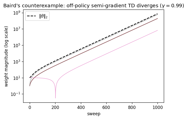
Any two are safe: tabular off-policy bootstrapping is Q-learning (Chapter 4, convergent); on-policy bootstrapping with approximation is Proposition 5.1; Monte Carlo with approximation and off-policy data is a genuine gradient method and is stable. All three together can make $\Pi_\mu\bellman^\policy$ — now with $\mu$ the wrong (off-policy) distribution — an expansion, and the parameters diverge to infinity. Baird Baird (1995) built the canonical witness.

The lesson is not that approximation is hopeless but that the interaction is what bites: the projected operator’s contraction was an on-policy privilege, and off-policy data revokes it. The next chapter’s engineering — target networks and replay — exists precisely to tame this instability well enough to train deep off-policy value functions in practice.

Beyond semi-gradient: LSTD and true-gradient methods

Two routes around the difficulty are worth naming. Least-squares TD (LSTD) solves the linear TD fixed-point equations directly: accumulate $A = \sum_t \phi(S_t)\big( \phi(S_t) - \discount\phi(S_{t+1})\big)^\top$ and $b = \sum_t \phi(S_t)R_{t+1}$, then set $\theta^\star = A^{-1}b$ — no step size, far more sample-efficient per datum, converging to the same on-policy fixed point as Proposition 5.1. Gradient-TD methods (GTD, TDC) instead descend a true objective (the projected Bellman error), restoring convergence even off-policy at the cost of a second set of weights. Both are the subject of the roadmap’s extension; LSTD appears in the companion.

The dynamic-programming bridge

Function approximation is the first crack in the contraction spine. Chapters 1–4 chased the unique fixed point of a $\discount$-contraction; here the object becomes $\Pi_\mu\bellman^\policy$, and its fixed point both moves (by the projection error) and, off-policy, may not exist as a stable limit at all. Two bridges forward:

• To control (LQR, Ch. 13). The linear-quadratic regulator is the lucky case where the optimal value is exactly quadratic — representable with zero projection error — so the approximation never bites and the Riccati recursion converges cleanly. Most of control’s tractable cases are exactly this: a function class the true value lives inside.
• To deep RL (Week 6). DQN keeps bootstrapping, off-policy data, and a (nonlinear) approximator — the full triad — and survives by engineering the instability down: a slowly-updated target network freezes the bootstrap target, and experience replay decorrelates and re-weights the update distribution toward something tamer.

What’s next

• Week 6 builds DQN: the replay buffer and target network as direct countermeasures to the deadly triad, scaling approximate value learning to pixels.

Exercises

1. (Derive) Write the semi-gradient TD(0) update for linear $V_\theta$ and show it is not the gradient of $\tfrac12\E[\delta_t^2]$. Identify the missing term.

   Solution

   $\nabla_\theta\tfrac12\delta_t^2 = \delta_t\nabla_\theta\delta_t = \delta_t\big( \discount\phi(S_{t+1}) - \phi(S_t)\big)$. Semi-gradient TD uses $-\delta_t\phi(S_t)$ (ascending $\delta_t\phi(S_t)$), dropping the $\discount\delta_t\phi(S_{t+1})$ term from differentiating the target. The dropped term is exactly what would make it a true gradient — and what, when present (residual-gradient methods), changes the fixed point and the stability.

2. (Prove) Show $\Pi_\mu\bellman^\policy$ is a $\discount$-contraction in $\norm{\cdot}_\mu$ when $\mu$ is the on-policy distribution, and derive the projection-error bound (Prop. 5.1).

   Solution

   $\bellman^\policy$ is a $\discount$-contraction in $\norm{\cdot}_\mu$ because $P_\policy$ is nonexpansive under the stationary $\mu$ (Jensen + $\mu^\top P_\policy = \mu^\top$); $\Pi_\mu$ is nonexpansive as an orthogonal projection; the composition is a $\discount$-contraction. The bound follows from $\Pi_\mu\valuefn_\policy = \Pi_\mu\bellman^\policy\valuefn_\policy$ and the triangle inequality, as in the proof above.

3. (Compute) In Baird’s setup the update is $\theta_{k+1} = (I + \alpha A)\theta_k$. What property of $A$ (or of $I + \alpha A$) causes divergence, and why does a small $\alpha$ not prevent it?

   Solution

   Divergence occurs iff $I + \alpha A$ has spectral radius $> 1$, i.e. $A$ has an eigenvalue with positive real part (for small $\alpha>0$, $\rho(I+\alpha A)>1$ exactly then). Shrinking $\alpha$ only slows the geometric blow-up; it cannot flip the sign of the unstable eigenvalue. The companion computes $A$‘s spectrum.

4. (Implement) Verify on the companion that on-policy semi-gradient TD converges to (near) $\valuefn_\policy$ on the random walk, while off-policy semi-gradient TD on Baird’s counterexample diverges (the committed figure).

   Solution

   See experiments/python/week05/test_fa.py: on-policy semi-gradient TD with tabular-complete features matches dp.policy_evaluation within a sampling tolerance and keeps bounded weights; Baird’s off-policy update grows the weight norm without bound (the divergence the figure plots).

5. (Extend) Implement LSTD and confirm it recovers the same on-policy fixed point as semi-gradient TD (and $\valuefn_\policy$ exactly when the features are tabular-complete).

   Solution

   LSTD solves $A\theta = b$ with $A = \sum_t\phi(S_t)(\phi(S_t)-\discount\phi(S_{t+1}))^\top$, $b=\sum_t\phi(S_t)R_{t+1}$; its solution is the TD fixed point. With tabular-complete features the projection error is zero and $\theta^\star$ reproduces $\valuefn_\policy$, which the companion’s lstd asserts against the Week-1 linear solve.

Companion code

The Week-5 companion lives at experiments/python/week05/ and reuses the Week-3 random walk and the Week-1 dp.policy_evaluation oracle. It is the chapter’s two poles side by side: a convergent on-policy method and a divergent off-policy one. (The roadmap suggests tile coding on MountainCar-v0; the random walk is used here because it has a closed-form $\valuefn_\policy$ to test against — MountainCar tile-coding is a natural deferred showcase that lacks an exact oracle.)

• fa.py — linear semi_gradient_td (constant step size with Polyak–Ruppert averaging) and lstd for a generic (P, R, policy) with an arbitrary feature matrix $\Phi$. Pure NumPy.
• baird.py — Baird’s seven-state counterexample: builds the feature matrix and the off-policy expected-update matrix $A$, iterates to divergence, and (with --plot) renders the committed divergence figure.
• test_fa.py — mathematical-correctness tests: on-policy semi-gradient TD converges to the analytic $\valuefn_\policy$ (and stays bounded); LSTD recovers $\valuefn_\policy$ with tabular-complete features; and Baird’s off-policy update diverges (the weight norm grows without bound while $A$ has an unstable eigenvalue).

# core algorithms + correctness tests (pure NumPy, no Gymnasium needed)
PYTHONPATH=. pytest experiments/python/week05/test_fa.py -q

# regenerate the committed Baird divergence figure
PYTHONPATH=. python experiments/python/week05/baird.py --plot