Model Predictive Control: Receding-Horizon Optimization as Implicit Feedback

Where we are. Chapter 13 solved the unconstrained linear-quadratic problem in closed form: one algebraic Riccati equation gives a single feedback gain $\lqrgain$ good for all time. But real actuators saturate, real states have limits, and the moment a constraint is present the Riccati equation has nothing to say — there is no closed form. Model predictive control (MPC) answers with a different idea: do not precompute one feedback law. Instead, at the current state, solve a finite-horizon optimal-control problem numerically, apply only its first move, and at the next state solve it again. The optimization is the controller — feedback by re-solving. This is the most widely deployed advanced control method in industry García et al. (1989) , and, read through Chapter 1, it is dynamic programming run online: an $\horizon$-step Bellman lookahead with the LQR cost-to-go grafted on as a terminal estimate.

From one gain to a horizon of decisions

Chapter 13 minimized a quadratic cost over an infinite horizon and got a stationary gain. MPC keeps the quadratic cost but makes three moves: it (i) truncates the horizon to a finite $\horizon$, (ii) adds hard constraints $\statevec_k\in\xset$, $u_k\in\uset$, and (iii) re-solves at every state rather than precomputing. The price of constraints is the loss of a closed form; the payment is a numerical optimization at each step — for linear dynamics and a quadratic cost, a quadratic program (QP), which modern solvers dispatch in microseconds Stellato et al. (2020) .

With $\xset,\uset,\termset$ polyhedral (box bounds, here), the problem is a convex QP: a quadratic objective in the stacked decision variables subject to linear equality (dynamics) and inequality (constraints) constraints.

The terminal cost that recovers LQR

Before stability, a sanity check that ties MPC to Chapter 13. Strip the constraints and set the terminal cost to the LQR cost-to-go. The finite horizon then collapses to the infinite-horizon answer — for any horizon length.

The terminal cost is doing the work: setting it to the exact optimal cost-to-go makes one step of lookahead see the entire infinite future, so the horizon length stops mattering.

Terminal ingredients

The recursive structure that made Proposition 15.1 work — appending the local LQR move at the end — is exactly what stability needs. Mayne et al. (2000) distilled it into two terminal ingredients: a terminal cost and a terminal set, compatible with a local controller (the textbook synthesis is Rawlings et al. (2017) ).

For the linear-quadratic problem there is a canonical choice: take $\kappa_f(\statevec)=-\lqrgain\statevec$ (the LQR law), $F(\statevec)=\statevec^\top\riccati\statevec$ (the DARE cost-to-go), and $\termset=\{\statevec:\statevec^\top\riccati\statevec\leq c\}$, the Lyapunov sublevel set on which $-\lqrgain\statevec$ respects the constraints. Condition (iii) then holds with equality: the DARE rearranges to $(\statemat-\inputmat\lqrgain)^\top\riccati(\statemat-\inputmat\lqrgain)-\riccati=-(Q+\lqrgain^\top R\lqrgain)$, which is exactly $F(\statevec^+)-F(\statevec)=-\ell(\statevec,-\lqrgain\statevec)$ along the local closed loop — the same Lyapunov identity proved in Chapter 13. Invariance follows from that identity: on $\termset$ the local closed loop gives $F(\statevec^+)\leq F(\statevec)\leq c$, so $\statevec^+\in\termset$; and constraint compatibility holds because $c$ is chosen small enough that $-\lqrgain\statevec$ stays within the input box — and, if a state box is present, $\termset$ within it — everywhere on $\termset$ (the companion’s terminal_region computes the largest such $c$, taking both bounds into account).

One caveat the companion makes concrete. The set $\termset=\{\statevec:\statevec^\top\riccati\statevec\leq c\}$ is quadratic, so imposing the terminal constraint $\statevec_\horizon\in\termset$ of Definition 15.1 literally would make the program a QCQP — which the QP solver OSQP cannot take. The companion therefore imposes the terminal cost (and, for the feasibility study, a linear terminal box as a concrete admissible surrogate for $\termset$) and verifies $\termset$-invariance of the realized closed loop rather than encoding it as a constraint. This suffices for the MPC$\equiv$LQR and stability demonstrations, which need only the terminal cost; the terminal-set constraint is what the general recursive-feasibility theorem below requires.

Stability: the value function is a Lyapunov function

With admissible terminal ingredients the descent argument of Chapter 14 transfers wholesale, but now the certificate is the optimization value $\mpcvalue$ itself. The engine is a single feasible candidate built by shifting the previous solution.

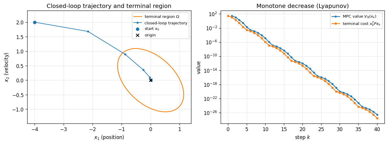
The proof is Chapter 14’s Lyapunov argument with $\lyap=\mpcvalue$, and the descent quantity is the stage cost — the same accounting as the LQR Lyapunov identity, now carried by the optimization rather than a fixed gain. The companion runs the closed loop on the double integrator and samples exactly this: the realized state goes to zero, $\mpcvalue$ is non-increasing step to step, the quadratic $\statevec^\top\riccati\statevec$ strictly decreases, and once the trajectory enters $\termset$ it never leaves.

Recursive feasibility

Stability assumed the problem stays solvable. That is not automatic — a feasible problem now can become infeasible next step if a constraint cannot be honored from the successor state. The shifted candidate of Lemma 15.1 settles it: it is a feasible plan at the successor, so feasibility propagates.

The growth of $\xset_\horizon$ with $\horizon$ is the practical knob: a state too far from the origin to be steered into the terminal region within a short horizon becomes reachable as the horizon lengthens. The companion demonstrates both directions — a tight terminal box with a far initial state is infeasible at a short horizon (the solver reports infeasibility and the code raises, never silently returning a bad move) and feasible once the horizon is long enough.

MPC as online approximate dynamic programming

This is the chapter the title promised. Set the two computations side by side.

• Chapter 1 (exact DP). The optimal cost-to-go solves the Bellman equation $\optvaluefn(\statevec)=\min_u[\,\ell(\statevec,u)+\optvaluefn(\statemat\statevec+\inputmat u)\,]$ (the deterministic, undiscounted cost form of Chapter 1’s $\optvaluefn=\bellmanopt\optvaluefn$), and the optimal policy is its one-step greedy minimizer. With constraints, $\optvaluefn$ has no closed form and the state space is continuous — exact DP is intractable.
• Chapter 15 (MPC). Replace the unknown tail $\optvaluefn$ by a finite unrolling plus a terminal estimate $F$: $\mpcvalue(\statevec)=\min[\sum_{k=0}^{\horizon-1}\ell(\statevec_k,u_k)+F(\statevec_\horizon)]$, and apply the one-step minimizer $\policy_\horizon(\statevec)=u_0^\star$.

MPC is therefore one Bellman step taken online, with the genuinely-optimal tail approximated by $\horizon-1$ exact steps and a terminal cost-to-go estimate. The horizon and the terminal estimate trade off: a perfect estimate needs no horizon (Proposition 15.1, where $F=\optvaluefn$ makes $\horizon=1$ exact), and a longer horizon forgives a cruder estimate. This is precisely “approximation in value space” — lookahead minimization over a terminal value approximation — the unifying view of Bertsekas’s reinforcement-learning-and-optimal-control program, which the convergence weeks take up directly (Week 19 reads MPC, rollout, and approximate policy iteration as one algorithm). The terminal cost is where a learned value function will later be grafted in: replace the LQR $\statevec^\top\riccati\statevec$ with a neural critic and MPC becomes a model-based RL controller — the MPC/RL hybrids of Part III. Chapter 13’s $\riccati$ is the value function; Chapter 14’s Lyapunov certificate is the terminal cost; Chapter 1’s Bellman step is the online minimization. Three chapters, one equation, now solved with constraints.

What’s next

• Week 16 (nonlinear and robust MPC). Drop linearity: the QP becomes a nonlinear program (direct multiple shooting, SQP/interior-point), and the terminal-ingredient theorem generalizes to the quasi-infinite-horizon scheme. Robust and tube MPC tighten constraints against disturbances to recover the guarantees this chapter proved only for the nominal model — closing the optimality-is-not-robustness gap. The recent-developments survey Mayne (2014) maps the territory.

Exercises

1. (Derive) Show that initializing the backward Riccati recursion at $\riccati_f=\riccati$ (the DARE solution) leaves every iterate equal to $\riccati$, and conclude the MPC law equals $-\lqrgain\statevec$ for all $\horizon$.

   Solution

   The DARE states $\riccati=Q+\statemat^\top\riccati\statemat-\statemat^\top\riccati\inputmat(R+\inputmat^\top\riccati\inputmat)^{-1}\inputmat^\top\riccati\statemat$, i.e. $\riccati$ is a fixed point of the Riccati map $\mathcal{R}$. The recursion is $\riccati_k=\mathcal{R}(\riccati_{k+1})$ with $\riccati_\horizon=\riccati$, so $\riccati_{\horizon-1}=\mathcal{R}(\riccati)=\riccati$ and by induction $\riccati_k=\riccati$ for all $k$. The first gain is then the stationary $\lqrgain$, so $u_0^\star=-\lqrgain\statevec$ independent of $\horizon$.

2. (Prove) Establish the value-descent inequality (Lemma 15.1) by constructing the shifted candidate and bounding its cost. Where is each terminal-ingredient axiom used?

   Solution

   With optimal $u^\star$ and states $\statevec_0,\dots,\statevec_\horizon$ at $\statevec$, take $\tilde u=(u_1^\star,\dots,u_{\horizon-1}^\star,\kappa_f(\statevec_\horizon))$ at $\statevec^+=\statevec_1$. Feasibility of the first $\horizon-1$ moves is inherited from $u^\star$; (i) and (ii) make the appended step feasible and keep the new terminal state in $\termset$. The cost of $\tilde u$ is $\mpcvalue(\statevec)-\ell(\statevec,u_0^\star)+F(\statevec_{\horizon+1})-F(\statevec_\horizon)+\ell(\statevec_\horizon,\kappa_f(\statevec_\horizon))$; axiom (iii) makes the last three terms $\leq0$. Since $\mpcvalue(\statevec^+)$ is the minimum, it is $\leq$ this candidate cost, giving the inequality.

3. (Compute) For a single-input system with DARE solution $\riccati$ and gain $\lqrgain$, find the largest $c$ such that $|{-}\lqrgain\statevec|\leq u_{\max}$ on the sublevel set $\{\statevec:\statevec^\top\riccati\statevec\leq c\}$.

   Solution

   Maximize $(\lqrgain\statevec)^2$ over $\statevec^\top\riccati\statevec\leq c$. With $y=\riccati^{1/2}\statevec$ the objective is $(\lqrgain\riccati^{-1/2}y)^2$ over $\norm{y}^2\leq c$, whose max is $c\,\lqrgain\riccati^{-1}\lqrgain^\top$ (Cauchy–Schwarz). Setting this $\leq u_{\max}^2$ gives $c=u_{\max}^2/(\lqrgain\riccati^{-1}\lqrgain^\top)$ — exactly the companion’s terminal_region.

4. (Implement) In the companion, verify the MPC$\equiv$LQR identity on both rails: the analytic condensed-QP solve to $10^{-9}$ and OSQP to $10^{-6}$, across several horizons and initial states.

   Solution

   See experiments/julia/week15/runtests.jl: with terminal cost $\riccati$ from dare_gain, kkt_solve_unconstrained returns $u_0=-\lqrgain\statevec_0$ to atol=1e-9 and solve_mpc (OSQP, polished, tight tolerances) to atol=1e-6, for $\horizon\in\{1,2,3,5,10,25\}$ and four initial states — Proposition 15.1 confirmed and the two-rail tolerance discipline made explicit.

5. (Extend) Demonstrate recursive feasibility numerically: pick a tight terminal box and a far initial state, show the short-horizon problem is infeasible and a long-horizon one feasible, and relate this to $\xset_\horizon\subseteq\xset_{\horizon+1}$.

   Solution

   See the companion’s feasibility test: from $\statevec_0=(10,0)$ with $|u|\leq1$ and terminal box $|\statevec_\horizon|\leq0.5$, solve_mpc raises at $\horizon=5$ (OSQP reports infeasible) and succeeds at $\horizon=40$, with the terminal box met. The far state is outside $\xset_5$ but inside $\xset_{40}$; since the feasible set grows with the horizon, lengthening it admits states a short horizon cannot steer into $\termset$ in time.

6. (Extend) Read MPC as one step of value iteration with an inexact terminal value. When is the first move exactly optimal for the infinite-horizon problem, and what does the gap between $F$ and $\optvaluefn$ cost?

   Solution

   MPC applies the greedy minimizer of $\sum_{k<\horizon}\ell+F(\statevec_\horizon)$, which is the $\horizon$-step Bellman lookahead with tail estimate $F$. If $F=\optvaluefn$ the lookahead is exact at $\horizon=1$ (Proposition 15.1 is the unconstrained instance, $F=\statevec^\top\riccati\statevec$). When $F\neq\optvaluefn$ — the generic constrained case — the first move is suboptimal for the infinite horizon by an amount that shrinks as $\horizon$ grows (more exact steps before the estimate is used) or as $F$ better approximates $\optvaluefn$. This is the approximation-in-value-space tradeoff Part III exploits by learning $F$.

Companion code

The Week-15 companion lives at experiments/julia/week15/ — the control lane is Julia-native from here (JuMP for modeling, OSQP for the QP), building on the tested dare_gain from experiments/julia/week13/. It pins the same discrete double-integrator literals as the Week-13 LQR suite, so the MPC results are parity-locked to the already-verified LQR/DARE base.

• mpc.jl — build_mpc_qp / solve_mpc (the OSQP rail; solve_mpc raises on any non-optimal termination); receding_horizon (closed-loop simulation recording the MPC value $\mpcvalue$); kkt_solve_unconstrained (the condensed dense solve — the $10^{-9}$ analytic rail); and terminal_region (the largest admissible sublevel-set $c$).
• runtests.jl — mathematical-correctness tests: the MPC$\equiv$LQR identity on both rails (Proposition 15.1); constraints binding with cost $\leq$ the saturated-LQR rollout; closed-loop stability with $\mpcvalue$ non-increasing, $\statevec^\top\riccati\statevec$ decreasing, and $\termset$ invariant (Lemma 15.1, Theorem 15.1); and recursive feasibility — infeasible at a short horizon, feasible at a long one (Theorem 15.2).

# linear-MPC companion: QP build/solve, two-rail parity, stability, feasibility
julia --project=experiments/julia experiments/julia/week15/runtests.jl

# the whole Julia control lane (weeks 11–15) in one aggregator run
make test-julia

The chapter figure is generated from the companion’s exported trajectory:

# export the closed-loop trajectory + terminal region, then render the figure
python experiments/python/week15/make_fig.py